w2dynamics: Frequency conventions and definitions

Introduction¶

w2dynamics is a software package for solving the single-impurity Anderson Model (SIAM) using continuous-time quantum Monte Carlo (CT-QMC) methods with the hybridization expansion (CT-HYB). It allows the calculation of local one- and two-particle quantities, such as the local Green’s function, self-energy, the two-particle Green’s function, and vertex functions. The documentation for w2dynamics provides some information on how to use the software, including installation instructions and very basic usage examples. The original publication associated with the package can be found here.

The many-body quantities described in the following are local $n$ -point (correlation) functions. Since DMFT only operates on a single lattice site, the spatial dependence of these quantities is trivial and can be dropped. However, these functions still include a subset of the following parameters for each leg: (Matsubara) frequency ( $\nu$ ), spin index ( $\sigma$ ), orbital index ( $o$ ) or imaginary time ( $\tau$ ). This introduces a huge amount of parameters appended to a variable and can be very cumbersome to read through if explicitly written down. Therefore, to increase readability, we follow Bickers et al., 1989 and group all indices that are not explicitly written down into a compound index, e.g. $\mathfrak{i}=\{o_i, \sigma_i, \nu_i\}$ . If an equation containing frequency or time-dependent quantities is written down with a compound index, it applies equally in both real and Fourier space. Furthermore, summing over these compound indices means summing over all individual components they include, with a normalization of $\frac 1\beta$ for frequency sums, where $\beta=\frac{1}{k_B T}$ is the inverse temperature.

Definitions¶

After this short introduction, let us state how w2dynamics defines the two-point (one-particle) Green’s function (in a system in thermal equilibrium):

\begin{align} G_{\mathfrak{12}}=-\left\langle\mathcal{T}\left [\hat{c}_{\mathfrak{1}}\hat{c}^{\dagger}_{\mathfrak{2}}\right ]\right\rangle\,. \end{align}

(1)

The two-particle Green’s function is defined as

\begin{align} G_{\mathfrak{1234}}=\left\langle\mathcal{T}\left [\hat{c}_{\mathfrak{1}}\hat{c}^{\dagger}_{\mathfrak{2}}\hat{c}_{\mathfrak{3}}\hat{c}^{\dagger}_{\mathfrak{4}}\right ]\right\rangle\,. \end{align}

(2)

Note that this operator ordering corresponds to the alternative convention for the four-point correlation function discussed in the section on basic definitions: here the odd (even) indices label annihilation (creation) operators, i.e. the mirror image of the ordering used elsewhere on this site.

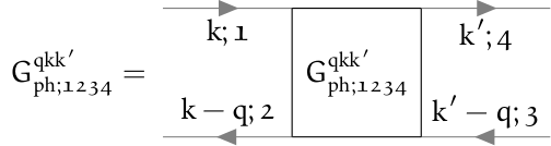
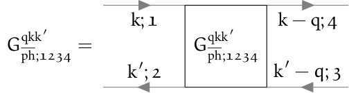
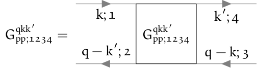
The frequency notation in all three channels ( $ph$ , $\overline{ph}$ , $pp$ ) is slightly different from the “Vienna” and “Munich” conventions as already mentioned at the beginning of the chapter.

\begin{align} \text{ph-notation:}&\;\;\{\nu_1=\nu,&&\nu_2=\nu-\omega,&&\nu_3=\nu'-\omega,&&\nu_4=\nu'\},\\ \overline{\text{ph}}\text{-notation:}&\;\;\{\nu_1=\nu,&&\nu_2=\nu',&&\nu_3=\nu'-\omega,&&\nu_4=\nu-\omega\}\quad\text{and}\\ \text{pp-notation:}&\;\;\{\nu_1=\nu,&&\nu_2=\omega-\nu',&&\nu_3=\omega-\nu,&&\nu_4=\nu'\}. \end{align}

(3)

The Fourier transform of the two-particle Green’s function in the $\text{ph}$ -channel is given by

\begin{align} G_{\text{ph}}(\nu,\nu',\omega)=\int_0^\beta \mathrm{d}^4\tau\; e^{i\nu(\tau_1-\tau_2)} e^{i\nu'(\tau_3-\tau_4)} e^{i\omega(\tau_2-\tau_3)} G(\tau_1,\tau_2,\tau_3,\tau_4)\,. \end{align}

(4)

The two-particle Green’s function in the three frequency conventions is diagrammatically shown below. The subscript $\{\text{ph},\overline{\text{ph}},\text{pp}\}$ denotes the frequency notation, not the channel reducibility, as G is reducible in all channels.

Crossing symmetries and frequency shifts¶

We will in the following show the frequency shifts needed to switch between different frequency notations for the two-particle Green’s function, which are the same as for the full vertex functions or the generalized susceptibilities.

\begin{align} G_{\text{ph};\mathfrak{1234}}^{\omega\nu\nu'} &=G_{\overline{\text{ph}};\mathfrak{1234}}^{(\nu-\nu')\nu(\nu-\omega)},\\ G_{\overline{\text{ph}};\mathfrak{1234}}^{\omega\nu\nu'}&=G_{\text{ph};\mathfrak{1234}}^{(\nu-\nu')\nu(\nu-\omega)},\\ G_{\text{ph};\mathfrak{1234}}^{\omega\nu\nu'} &=G_{\text{pp};\mathfrak{1234}}^{(\nu+\nu'-\omega)\nu\nu'}\quad\text{and}\\ G_{\text{pp};\mathfrak{1234}}^{\omega\nu\nu'} &=G_{\text{ph};\mathfrak{1234}}^{(\nu+\nu'-\omega)\nu\nu'}. \end{align}

(5)

The crossing symmetries for the two-particle Green’s function in w2dynamics’ convention (in $\text{ph}$ notation) read

\begin{align} G_{\text{ph};\sigma\sigma';\mathfrak{1234}}^{\omega\nu\nu'} = -G_{\text{ph};\sigma'\sigma;\mathfrak{3214}}^{(\nu'-\nu)(\nu'-\omega)\nu'} = G_{\text{ph};\sigma'\sigma;\mathfrak{3412}}^{(-\omega)(\nu'-\omega)(\nu-\omega)} = -G_{\text{ph};\sigma\sigma';\mathfrak{1432}}^{(\nu-\nu')\nu(\nu-\omega)}\,. \end{align}

(6)

Connected two-particle Green’s function and vertex function¶

Let us finally note that the two-particle Green’s function represents all diagrams that are possible that involve two electrons, two holes or an electron and a hole. It can therefore be split into two parts: (i) a part, where the electrons do not interact with each other and propagate independently; and (ii) a part, where the electrons do interact with each other through an infinite number of processes. Part (ii) is commonly called the connected two-particle Green’s function and can be obtained by removing the disconnected parts (i) from the full Green’s function

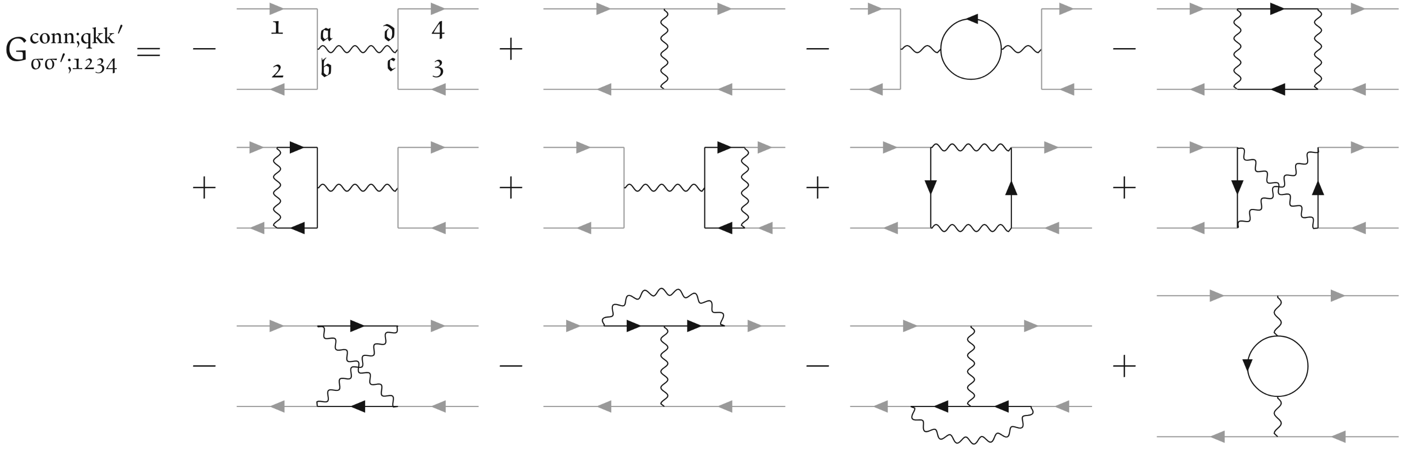
\begin{align} G_{\sigma\sigma';\mathfrak{1234}}^{\omega\nu\nu'}=G_{\sigma\sigma';\mathfrak{1234}}^{\text{conn};\omega\nu\nu'}+\delta_{\omega 0}G_{\sigma;\mathfrak{12}}^{\nu}G_{\sigma';\mathfrak{34}}^{\nu'}-\delta_{\sigma\sigma'}\delta_{\nu\nu'}G_{\sigma;\mathfrak{14}}^{\nu}G_{\sigma;\mathfrak{32}}^{\nu-\omega}. \end{align}

(7)

Diagrammatically, the connected two-particle Green’s function contains all diagrams, where two propagating electrons interact with each other. The first terms up to interaction order two are shown below.

The disconnected part only contains the non-interacting diagrams, where the two electrons propagate independently,

The full vertex¶

Lastly, the full vertex function $F$ is defined as the connected two-particle Green’s function with the external legs removed, i.e. amputated:

\begin{align} G_{\mathfrak{1234}}^{\text{conn};\omega\nu\nu'} = -\frac1\beta \sum_{\mathfrak{abcd}} G_{\mathfrak{1a}}^{\nu} G_{\mathfrak{b2}}^{\nu-\omega} F_{\mathfrak{abcd}}^{\omega\nu\nu'} G_{\mathfrak{3c}}^{\nu'-\omega} G_{\mathfrak{d4}}^{\nu'}. \end{align}

(8)

References¶

Wallerberger, M., Hausoel, A., Gunacker, P., Kowalski, A., Parragh, N., Goth, F., Held, K., & Sangiovanni, G. (2019). w2dynamics: Local one- and two-particle quantities from dynamical mean field theory. Computer Physics Communications, 235, 388–399. 10.1016/j.cpc.2018.09.007
Bickers, N. E., Scalapino, D. J., & White, S. R. (1989). Conserving Approximations for Strongly Correlated Electron Systems: Bethe-Salpeter Equation and Dynamics for the Two-Dimensional Hubbard Model. Physical Review Letters, 62(8), 961–964. 10.1103/physrevlett.62.961
Peil, J. (2025). Multi-orbital dynamical vertex approximation. 10.34726/HSS.2025.130528