Two-particle QFT in the real-frequency Keldysh formalism
Alternatively to the imaginary-time (Matsubara) formalism used on the other pages, two-particle quantum field theory can also be formulated in the real-frequency Keldysh formalism. This is particularly useful for studying non-equilibrium steady states, but can also be applied to equilibrium situations, avoiding the need for analytic continuation from imaginary to real frequencies.
Here, we will only discuss the Keldysh formalism in the steady state, which permits a Fourier transform from time to frequency space. In time-dependent situations, the two-particle quantities depend on more complicated time arguments (e.g., two-particle Green’s functions depend on four time arguments), which makes the treatment more involved. We do not discuss this case here.
Many-body action in the Keldysh formalism ¶ We begin again with the many-body Hamiltonian in second quantization. In the Keldysh formalism, the partition function is given by the path integral
Z = ∫ D [ c ˉ , c ] e i S [ c ˉ , c ] S [ c ˉ , c ] = ∫ C d t { ∑ 1 c ˉ 1 ( t ) i ∂ t c 1 ( t ) − H [ c 1 † ( t ) , c ( t ) ] } = S 0 + S I , \begin{align}
Z &= \int \mathcal{D}[\bar{c}, c] \,e^{i S[\bar{c}, c]} \\
S[\bar{c}, c] &= \int_\mathcal{C} dt \left\{ \sum_1 \bar{c}_1(t) i \partial_t c_1(t) - H[c_1^\dagger(t), c(t)] \right\} = S_0 + S_I \, ,
\end{align} Z S [ c ˉ , c ] = ∫ D [ c ˉ , c ] e i S [ c ˉ , c ] = ∫ C d t { 1 ∑ c ˉ 1 ( t ) i ∂ t c 1 ( t ) − H [ c 1 † ( t ) , c ( t )] } = S 0 + S I , where the time integral runs along the Keldysh contour C \mathcal{C} C t = − ∞ t=-\infty t = − ∞ t = + ∞ t=+\infty t = + ∞ c ˉ 1 ( t ) \bar{c}_1(t) c ˉ 1 ( t ) c 1 ( t ) c_1(t) c 1 ( t )
For an arbitrary quartic interaction, we can write the action as
S = S 0 + S I = c ‾ 1 ( G 0 − 1 ) 12 c 2 + 1 4 c ‾ 1 c ‾ 3 F 0 , 1234 c 2 c 4 , \begin{align}
S = S_0 + S_I = \overline{c}_1 (G_0^{-1})_{12} c_2 + \frac{1}{4} \overline{c}_1 \overline{c}_3 F_{0,1234} c_2 c_4 \, ,
\end{align} S = S 0 + S I = c 1 ( G 0 − 1 ) 12 c 2 + 4 1 c 1 c 3 F 0 , 1234 c 2 c 4 , where repeated indices imply summation/integration. Here, G 0 G_0 G 0 F 0 F_0 F 0
Correlation functions ¶ The two-point and four-point correlation functions are defined as in the Matsubara formalism, with an additional contour-ordering operator T C \mathcal{T}_\mathcal{C} T C i i i
G 21 = − i ⟨ T C c 2 c ‾ 1 ⟩ , G 4231 ( 4 ) = i ⟨ T C c 4 c 2 c ‾ 3 c ‾ 1 ⟩ . \begin{align}
G_{21} &= -i \langle \mathcal{T}_\mathcal{C} c_2 \overline{c}_1 \rangle \, , \\
G^{(4)}_{4231} &= i \langle \mathcal{T}_\mathcal{C} c_4 c_2 \overline{c}_3 \overline{c}_1 \rangle \, .
\end{align} G 21 G 4231 ( 4 ) = − i ⟨ T C c 2 c 1 ⟩ , = i ⟨ T C c 4 c 2 c 3 c 1 ⟩ . The factors of i i i
Z [ J ˉ , J ] = ∫ D [ c ˉ , c ] e i S [ c ˉ , c ] + i J ˉ c + i c ‾ J . \begin{align}
Z[\bar{J}, J] = \int \mathcal{D}[\bar{c}, c] \,e^{i S[\bar{c}, c] + i \bar{J} c + i \overline{c} J} \, .
\end{align} Z [ J ˉ , J ] = ∫ D [ c ˉ , c ] e i S [ c ˉ , c ] + i J ˉ c + i c J . Now, due to the factor of i i i i i i
δ δ J ˉ ↔ i c ; δ δ J ↔ i c ‾ . \begin{align}
\frac{\delta}{\delta \bar{J}} &\leftrightarrow i c \, ; & \frac{\delta}{\delta J} &\leftrightarrow i \overline{c} \, .
\end{align} δ J ˉ δ ↔ i c ; δ J δ ↔ i c . Hence, a contour-ordered 2 n 2n 2 n 1 / i ( 2 n ) 1/i^{(2n)} 1/ i ( 2 n )
⟨ T C c 1 … c n c ‾ n + 1 … c ‾ 2 n ⟩ = 1 i 2 n 1 Z δ 2 n Z δ J ˉ 1 … δ J ˉ n δ J n + 1 … δ J 2 n ∣ J ˉ = J = 0 . \begin{align}
\langle T_\mathcal{C} c_1 \ldots c_n \overline{c}_{n+1} \ldots \overline{c}_{2n} \rangle = \frac{1}{i^{2n}} \frac{1}{Z} \frac{\delta^{2n} Z}{\delta \bar{J}_1 \ldots \delta \bar{J}_n \delta J_{n+1} \ldots \delta J_{2n}} \Bigg|_{\bar{J}=J=0} \, .
\end{align} ⟨ T C c 1 … c n c n + 1 … c 2 n ⟩ = i 2 n 1 Z 1 δ J ˉ 1 … δ J ˉ n δ J n + 1 … δ J 2 n δ 2 n Z ∣ ∣ J ˉ = J = 0 . Now, for an interacting theory, such computations cannot be done exactly. But we can do them for a non-interacting theory, for which we can compute the Gaussian path integral. The generating functional for the non-interacting theory reads
Z 0 [ J ˉ , J ] = ∫ D [ c ˉ , c ] e i c ˉ ( G 0 − 1 ) c + i J ˉ c + i c ‾ J = Z 0 [ 0 , 0 ] e − i J ˉ G 0 J , \begin{align}
Z_0[\bar{J}, J] &= \int \mathcal{D}[\bar{c}, c] \,e^{i \bar{c} (G_0^{-1}) c + i \bar{J} c + i \overline{c} J} \\
&= Z_0[0,0] \, e^{-i \bar{J} G_0 J} \, ,
\end{align} Z 0 [ J ˉ , J ] = ∫ D [ c ˉ , c ] e i c ˉ ( G 0 − 1 ) c + i J ˉ c + i c J = Z 0 [ 0 , 0 ] e − i J ˉ G 0 J , where Z 0 [ 0 , 0 ] Z_0[0,0] Z 0 [ 0 , 0 ] − i G 0 -i G_0 − i G 0
δ 2 Z 0 [ J ˉ , J ] δ J ˉ δ J = ( − i ) G 0 Z 0 . \begin{align}
\frac{\delta^2 Z_0[\bar{J}, J]}{\delta \bar{J} \delta J} &= (-i) G_{0} Z_0 \, .
\end{align} δ J ˉ δ J δ 2 Z 0 [ J ˉ , J ] = ( − i ) G 0 Z 0 . We hence find that the two-point correlation function is given by
⟨ T C c c ‾ ⟩ 0 = 1 i 2 ( − i ) G 0 = i G 0 ⇔ G 0 = − i ⟨ T C c c ‾ ⟩ 0 . \begin{align}
\langle T_\mathcal{C} c \overline{c} \rangle_0 = \frac{1}{i^2} (-i) G_0 = i G_0 \ \Leftrightarrow \ G_0 = -i \langle T_\mathcal{C} c \overline{c} \rangle_0 \, .
\end{align} ⟨ T C c c ⟩ 0 = i 2 1 ( − i ) G 0 = i G 0 ⇔ G 0 = − i ⟨ T C c c ⟩ 0 . By analogy, we demand the same normalization for the interacting theory.
For higher-point correlation functions, the situation is not so clear and indeed different conventions exist in the literature. Here, we follow the commonly used convention that an n n n ( − i ) ( n − 1 ) (-i)^{(n-1)} ( − i ) ( n − 1 )
As a consequence, the tree expansion of the four-point correlation function reads
i G 4231 ( 4 ) = G 41 G 23 + ζ G 43 G 21 + i G c , 4321 ( 4 ) , \begin{align}
iG^{(4)}_{4231} = G_{41} G_{23} + \zeta G_{43} G_{21} + i G^{(4)}_{c,4321}\, ,
\end{align} i G 4231 ( 4 ) = G 41 G 23 + ζ G 43 G 21 + i G c , 4321 ( 4 ) , with the connected part given by
G c , 4321 ( 4 ) = − G 4 1 ~ G 2 3 ~ F 1 ~ 2 ~ 3 ~ 4 ~ G 2 ~ 3 G 4 ~ 1 . \begin{align}
G^{(4)}_{c,4321} = - G_{4\tilde{1}} G_{2\tilde{3}} F_{\tilde{1}\tilde{2}\tilde{3}\tilde{4}} G_{\tilde{2}3} G_{\tilde{4}1}\, .
\end{align} G c , 4321 ( 4 ) = − G 4 1 ~ G 2 3 ~ F 1 ~ 2 ~ 3 ~ 4 ~ G 2 ~ 3 G 4 ~ 1 . For the disconnected terms, this form of the tree-expansion is motivated by the non-interacting case, where Wick’s theorem gives
G 0 , 4321 ( 4 ) = i ⟨ T C c 4 c 2 c ‾ 3 c ‾ 1 ⟩ 0 = i ( ⟨ T C c 4 c ˉ 1 ⟩ 0 ⟨ T C c 2 c ˉ 3 ⟩ 0 + ζ ⟨ T C c 4 c ˉ 3 ⟩ 0 ⟨ T C c 2 c ˉ 1 ⟩ 0 ) = i ( i G 0 , 41 i G 0 , 23 + ζ i G 0 , 43 i G 0 , 21 ) = − i ( G 0 , 41 G 0 , 23 + ζ G 0 , 43 G 0 , 21 ) ⇔ i G 0 , 4321 ( 4 ) = G 0 , 41 G 0 , 23 + ζ G 0 , 43 G 0 , 21 . \begin{align}
G^{(4)}_{0, 4321} &= i \langle T_\mathcal{C} c_4 c_2 \overline{c}_3 \overline{c}_1 \rangle_0 = i \left( \langle T_\mathcal{C} c_4 \bar{c}_1\rangle_0 \langle T_\mathcal{C} c_2 \bar{c}_3\rangle_0 + \zeta \langle T_\mathcal{C} c_4 \bar{c}_3\rangle_0 \langle T_\mathcal{C} c_2 \bar{c}_1\rangle_0 \right) \\
&= i \left( i G_{0,41} i G_{0,23} + \zeta i G_{0,43} i G_{0,21} \right) = -i \left( G_{0,41} G_{0,23} + \zeta G_{0,43} G_{0,21} \right) \\ & \\
\Leftrightarrow \quad i G^{(4)}_{0, 4321} &= G_{0,41} G_{0,23} + \zeta G_{0,43} G_{0,21} \, .
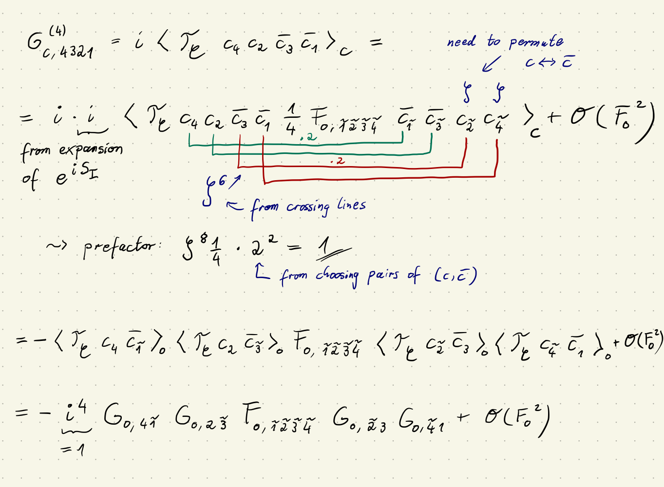
\end{align} G 0 , 4321 ( 4 ) ⇔ i G 0 , 4321 ( 4 ) = i ⟨ T C c 4 c 2 c 3 c 1 ⟩ 0 = i ( ⟨ T C c 4 c ˉ 1 ⟩ 0 ⟨ T C c 2 c ˉ 3 ⟩ 0 + ζ ⟨ T C c 4 c ˉ 3 ⟩ 0 ⟨ T C c 2 c ˉ 1 ⟩ 0 ) = i ( i G 0 , 41 i G 0 , 23 + ζ i G 0 , 43 i G 0 , 21 ) = − i ( G 0 , 41 G 0 , 23 + ζ G 0 , 43 G 0 , 21 ) = G 0 , 41 G 0 , 23 + ζ G 0 , 43 G 0 , 21 . The sign of the connected part is best motivated by the first-order contribution in perturbation theory in the bare interaction F 0 F_0 F 0
Keldysh index structure of two- and four-point functions ¶ Since a general n n n n n n 2 n 2^n 2 n
Propagator ¶ Starting, with the two-point Green’s function, we can arrange its four Keldysh components in a 2 × 2 2\times 2 2 × 2
( G c 2 c 1 ) = ( G − − G − + G + − G + + ) , \begin{align}
(G^{c_2 c_1}) =
\begin{pmatrix}
G^{--} & G^{-+} \\
G^{+-} & G^{++}
\end{pmatrix} \, ,
\end{align} ( G c 2 c 1 ) = ( G −− G +− G −+ G ++ ) , where the superscripts c 2 , c 1 ∈ { − , + } c_2, c_1 \in \{-, +\} c 2 , c 1 ∈ { − , + }
G − ∣ + ( t 2 , t 1 ) = − i ⟨ T C c − ( t 2 ) c ‾ + ( t 1 ) ⟩ = − ζ i ⟨ c ‾ ( t 1 ) c ( t 2 ) ⟩ ≡ G < ( t 2 , t 1 ) G + ∣ − ( t 2 , t 1 ) = − i ⟨ T C c + ( t 2 ) c ‾ − ( t 1 ) ⟩ = − i ⟨ c ( t 2 ) c ‾ ( t 1 ) ⟩ ≡ G > ( t 2 , t 1 ) G − − ( t 2 , t 1 ) = − i ⟨ T C c − ( t 2 ) c ‾ − ( t 1 ) ⟩ = G > ( t 2 , t 1 ) θ ( t 2 − t 1 ) + G < ( t 2 , t 1 ) θ ( t 1 − t 2 ) G + + ( t 2 , t 1 ) = − i ⟨ T C c + ( t 2 ) c ‾ + ( t 1 ) ⟩ = G < ( t 2 , t 1 ) θ ( t 2 − t 1 ) + G > ( t 2 , t 1 ) θ ( t 1 − t 2 ) , \begin{align}
G^{-|+}(t_2, t_1) &= -i \langle \mathcal{T}_\mathcal{C} c^-(t_2) \overline{c}^+(t_1) \rangle = - \zeta i \langle \overline{c}(t_1) c(t_2) \rangle \equiv G^<(t_2, t_1) \\
G^{+|-}(t_2, t_1) &= -i \langle \mathcal{T}_\mathcal{C} c^+(t_2) \overline{c}^-(t_1) \rangle = -i \langle c(t_2) \overline{c}(t_1) \rangle \equiv G^>(t_2, t_1) \\
G^{--}(t_2, t_1) &= -i \langle \mathcal{T}_{\mathcal{C}} c^-(t_2) \overline{c}^-(t_1) \rangle = G^>(t_2, t_1) \theta(t_2 - t_1) + G^<(t_2, t_1) \theta(t_1 - t_2) \\
G^{++}(t_2, t_1) &= -i \langle \mathcal{T}_{\mathcal{C}} c^+(t_2) \overline{c}^+(t_1) \rangle = G^<(t_2, t_1) \theta(t_2 - t_1) + G^>(t_2, t_1) \theta(t_1 - t_2) \, ,
\end{align} G − ∣ + ( t 2 , t 1 ) G + ∣ − ( t 2 , t 1 ) G −− ( t 2 , t 1 ) G ++ ( t 2 , t 1 ) = − i ⟨ T C c − ( t 2 ) c + ( t 1 )⟩ = − ζ i ⟨ c ( t 1 ) c ( t 2 )⟩ ≡ G < ( t 2 , t 1 ) = − i ⟨ T C c + ( t 2 ) c − ( t 1 )⟩ = − i ⟨ c ( t 2 ) c ( t 1 )⟩ ≡ G > ( t 2 , t 1 ) = − i ⟨ T C c − ( t 2 ) c − ( t 1 )⟩ = G > ( t 2 , t 1 ) θ ( t 2 − t 1 ) + G < ( t 2 , t 1 ) θ ( t 1 − t 2 ) = − i ⟨ T C c + ( t 2 ) c + ( t 1 )⟩ = G < ( t 2 , t 1 ) θ ( t 2 − t 1 ) + G > ( t 2 , t 1 ) θ ( t 1 − t 2 ) , where we have suppressed all other dependencies for ease of notation. Here, the contour-time-ordering has been made explicit and the greater and lesser Green’s functions G > G^> G > G < G^< G <
As can be confirmed by direct calculation, the four Keldysh components are not independent, but satisfy the relation
G − ∣ + + G + ∣ − = G − − + G + + . \begin{align}
G^{-|+} + G^{+|-} = G^{--} + G^{++} \, .
\end{align} G − ∣ + + G + ∣ − = G −− + G ++ . Making use of this redundancy motivates the Keldysh rotation , defined as
G k 2 k 1 = D k 2 c 2 G c 2 c 1 ( D − 1 ) c 1 k 1 , \begin{align}
G^{k_2 k_1} = D^{k_2 c_2} G^{c_2 c_1} (D^{-1})^{c_1 k_1} \, ,
\end{align} G k 2 k 1 = D k 2 c 2 G c 2 c 1 ( D − 1 ) c 1 k 1 , with the transformation matrix
D = 1 2 ( 1 − 1 1 1 ) ; D − 1 = 1 2 ( 1 1 − 1 1 ) . \begin{align}
D &= \frac{1}{\sqrt{2}}
\begin{pmatrix}
1 & -1 \\
1 & 1
\end{pmatrix}\, ; &
D^{-1} &= \frac{1}{\sqrt{2}}
\begin{pmatrix}
1 & 1 \\
-1 & 1
\end{pmatrix} \, .
\end{align} D = 2 1 ( 1 1 − 1 1 ) ; D − 1 = 2 1 ( 1 − 1 1 1 ) . The Keldysh-rotated Green’s function then takes the form
( G k 2 k 1 ) = ( 0 G A G R G K ) , \begin{align}
(G^{k_2 k_1}) =
\begin{pmatrix}
0 & G^A \\
G^R & G^K
\end{pmatrix} \, ,
\end{align} ( G k 2 k 1 ) = ( 0 G R G A G K ) , where the component G 11 G^{11} G 11 G R ( t 2 , t 1 ) = − i ⟨ [ c ( t 2 ) , c ‾ ( t 1 ) ] ζ ⟩ θ ( t 2 − t 1 ) G^R(t_2, t_1) = -i \langle [c(t_2), \overline{c}(t_1)]_\zeta \rangle \theta(t_2 - t_1) G R ( t 2 , t 1 ) = − i ⟨[ c ( t 2 ) , c ( t 1 ) ] ζ ⟩ θ ( t 2 − t 1 ) retarded Green’s function , G A ( t 2 , t 1 ) = [ G R ( t 1 , t 2 ) ] ∗ G^A(t_2, t_1) = [G^R(t_1, t_2)]^* G A ( t 2 , t 1 ) = [ G R ( t 1 , t 2 ) ] ∗ advanced component, and G K ( t 2 , t 1 ) = G > ( t 2 , t 1 ) + G < ( t 2 , t 1 ) = − [ G K ( t 1 , t 2 ) ] ∗ G^K(t_2, t_1) = G^>(t_2, t_1) + G^<(t_2, t_1) = -[G^K(t_1, t_2)]^* G K ( t 2 , t 1 ) = G > ( t 2 , t 1 ) + G < ( t 2 , t 1 ) = − [ G K ( t 1 , t 2 ) ] ∗ Keldysh component.
Bubble ¶ This Keldysh structure of the propagator carries over to the bubble
χ 0 k 4 , k 3 , k 2 , k 1 = G k 4 k 1 G k 2 k 3 . \begin{align}
\chi_0^{k_4, k_3, k_2, k_1} = G^{k_4 k_1} G^{k_2 k_3} \, .
\end{align} χ 0 k 4 , k 3 , k 2 , k 1 = G k 4 k 1 G k 2 k 3 . Formally organizing the 16 Keldysh components in a 4 × 4 4\times 4 4 × 4
( χ 0 k 4 k 3 k 2 k 1 ) = ( 1111 1112 1121 1122 1211 1212 1221 1222 2111 2112 2121 2122 2211 2212 2221 2222 ) = ( G 11 G 11 G 12 G 11 G 11 G 21 G 12 G 21 G 11 G 12 G 12 G 12 G 11 G 22 G 12 G 22 G 21 G 11 G 22 G 11 G 21 G 21 G 22 G 21 G 21 G 12 G 22 G 12 G 21 G 22 G 22 G 22 ) = ( 0 0 0 G A G R 0 G A G A 0 G A G K 0 0 G R G R G K G R G R G A G K G A G R G K G K G K ) . \begin{align}
(\chi_0^{k_4 k_3 k_2 k_1}) &=
\begin{pmatrix}
1111 & 1112 & 1121 & 1122 \\
1211 & 1212 & 1221 & 1222 \\
2111 & 2112 & 2121 & 2122 \\
2211 & 2212 & 2221 & 2222
\end{pmatrix} \\
&=
\begin{pmatrix}
G^{11} G^{11} & G^{12} G^{11} & G^{11} G^{21} & G^{12} G^{21} \\
G^{11} G^{12} & G^{12} G^{12} & G^{11} G^{22} & G^{12} G^{22} \\
G^{21} G^{11} & G^{22} G^{11} & G^{21} G^{21} & G^{22} G^{21} \\
G^{21} G^{12} & G^{22} G^{12} & G^{21} G^{22} & G^{22} G^{22}
\end{pmatrix} \\
&=
\begin{pmatrix}
0 & 0 & 0 & G^A G^R \\
0 & G^A G^A & 0 & G^A G^K \\
0 & 0 & G^R G^R & G^K G^R \\
G^R G^A & G^K G^A & G^R G^K & G^K G^K
\end{pmatrix}\, .
\end{align} ( χ 0 k 4 k 3 k 2 k 1 ) = ⎝ ⎛ 1111 1211 2111 2211 1112 1212 2112 2212 1121 1221 2121 2221 1122 1222 2122 2222 ⎠ ⎞ = ⎝ ⎛ G 11 G 11 G 11 G 12 G 21 G 11 G 21 G 12 G 12 G 11 G 12 G 12 G 22 G 11 G 22 G 12 G 11 G 21 G 11 G 22 G 21 G 21 G 21 G 22 G 12 G 21 G 12 G 22 G 22 G 21 G 22 G 22 ⎠ ⎞ = ⎝ ⎛ 0 0 0 G R G A 0 G A G A 0 G K G A 0 0 G R G R G R G K G A G R G A G K G K G R G K G K ⎠ ⎞ . Self-energy ¶ The Keldysh rotation can be applied to the self-energy, Σ k 1 k 2 = D k 1 c 1 Σ c 1 c 2 ( D − 1 ) c 2 k 1 \Sigma^{k_1 k_2} = D^{k_1 c_1} \Sigma^{c_1 c_2} (D^{-1})^{c_2 k_1} Σ k 1 k 2 = D k 1 c 1 Σ c 1 c 2 ( D − 1 ) c 2 k 1
( Σ k 1 k 2 ) = ( Σ K Σ R Σ A 0 ) . \begin{align}
(\Sigma^{k_1 k_2}) =
\begin{pmatrix}
\Sigma^{K} & \Sigma^{R} \\
\Sigma^{A} & 0
\end{pmatrix} \, .
\end{align} ( Σ k 1 k 2 ) = ( Σ K Σ A Σ R 0 ) . Due to causality, the component Σ 22 \Sigma^{22} Σ 22 G G G k 1 k_1 k 1 k 2 k_2 k 2
This fact can be most easily motivated by looking at the Dyson equation in the form G − 1 = G 0 − 1 − Σ G^{-1} = G_0^{-1} - \Sigma G − 1 = G 0 − 1 − Σ 2 × 2 2\times 2 2 × 2
( 0 A R K ) − 1 = 1 0 ⋅ K − A R ( K − A − R 0 ) = ( − A − 1 K R − 1 R − 1 A − 1 0 ) , \begin{align}
\begin{pmatrix}
0 & A \\
R & K
\end{pmatrix}^{-1} =
\frac{1}{0\cdot K - A R}
\begin{pmatrix}
K & -A \\
-R & 0
\end{pmatrix} =
\begin{pmatrix}
-A^{-1} K R^{-1} & R^{-1} \\
A^{-1} & 0
\end{pmatrix} \, ,
\end{align} ( 0 R A K ) − 1 = 0 ⋅ K − A R 1 ( K − R − A 0 ) = ( − A − 1 K R − 1 A − 1 R − 1 0 ) , the positions of the retarded and advanced components are swapped, and the other non-trivial component is the 1 × 1 1\times 1 1 × 1
Dyson equation ¶ Speaking of the Dyson equation, which reads in its most general form
G = G 0 + G 0 ∘ Σ ∘ G , \begin{align}
G = G_0 + G_0 \circ \Sigma \circ G \, ,
\end{align} G = G 0 + G 0 ∘ Σ ∘ G , where the connector ∘ denotes contractions in time and single-particle quantum numbers. Making the Keldysh structure explicit, separate Dyson equations for the individual Keldysh components can be derived. They read
G R = G 0 R + G 0 R ∙ Σ R ∙ G R , G A = G 0 A + G 0 A ∙ Σ A ∙ G A , G K = ( 1 + G R ∙ Σ R ) ∙ G 0 K ∙ ( 1 + Σ A ∙ G A ) + G R ∙ Σ K ∙ G A , \begin{align}
G^{R} &= G_0^{R} + G_0^{R} \bullet \Sigma^{R} \bullet G^{R} \, , \\
G^{A} &= G_0^{A} + G_0^{A} \bullet \Sigma^{A} \bullet G^{A} \, , \\
G^{K} &= (1 + G^{R} \bullet \Sigma^{R}) \bullet G_0^{K} \bullet (1 + \Sigma^{A} \bullet G^{A}) + G^{R} \bullet \Sigma^{K} \bullet G^{A} \, ,
\end{align} G R G A G K = G 0 R + G 0 R ∙ Σ R ∙ G R , = G 0 A + G 0 A ∙ Σ A ∙ G A , = ( 1 + G R ∙ Σ R ) ∙ G 0 K ∙ ( 1 + Σ A ∙ G A ) + G R ∙ Σ K ∙ G A , where the bullet ∙ \bullet ∙
To derive these equations, we start from the general Dyson equation written explicitly in Keldysh space,
( 0 G A G R G K ) = ( 0 G 0 A G 0 R G 0 K ) + ( 0 G 0 A G 0 R G 0 K ) ∙ ( Σ K Σ R Σ A 0 ) ∙ ( 0 G A G R G K ) = ( 0 G 0 A G 0 R G 0 K ) + ( 0 G 0 A ∙ Σ A ∙ G A G 0 R ∙ Σ R ∙ G R ( G 0 R ∙ Σ K + G 0 K ∙ Σ A ) ∙ G A + G 0 R ∙ Σ R ∙ G K ) . \begin{align}
\begin{pmatrix}
0 & G^{A} \\
G^{R} & G^{K}
\end{pmatrix} &=
\begin{pmatrix}
0 & G_0^{A} \\
G_0^{R} & G_0^{K}
\end{pmatrix} +
\begin{pmatrix}
0 & G_0^{A} \\
G_0^{R} & G_0^{K}
\end{pmatrix} \bullet
\begin{pmatrix}
\Sigma^{K} & \Sigma^{R} \\
\Sigma^{A} & 0
\end{pmatrix} \bullet
\begin{pmatrix}
0 & G^{A} \\
G^{R} & G^{K}
\end{pmatrix} \\
&= \begin{pmatrix}
0 & G_0^{A} \\
G_0^{R} & G_0^{K}
\end{pmatrix} +
\begin{pmatrix}
0 & G_0^{A} \bullet \Sigma^{A} \bullet G^{A} \\
G_0^{R} \bullet \Sigma^{R} \bullet G^{R} & (G_0^{R} \bullet \Sigma^{K} + G_0^{K} \bullet \Sigma^{A}) \bullet G^{A} + G_0^{R} \bullet \Sigma^{R} \bullet G^{K}
\end{pmatrix} \, .
\end{align} ( 0 G R G A G K ) = ( 0 G 0 R G 0 A G 0 K ) + ( 0 G 0 R G 0 A G 0 K ) ∙ ( Σ K Σ A Σ R 0 ) ∙ ( 0 G R G A G K ) = ( 0 G 0 R G 0 A G 0 K ) + ( 0 G 0 R ∙ Σ R ∙ G R G 0 A ∙ Σ A ∙ G A ( G 0 R ∙ Σ K + G 0 K ∙ Σ A ) ∙ G A + G 0 R ∙ Σ R ∙ G K ) . We directly obtain the two independent Dyson equations for the retarded and advanced components,
G R = G 0 R + G 0 R ∙ Σ R ∙ G R , G A = G 0 A + G 0 A ∙ Σ A ∙ G A , \begin{align}
G^{R} &= G_0^{R} + G_0^{R} \bullet \Sigma^{R} \bullet G^{R} \, , \\
G^{A} &= G_0^{A} + G_0^{A} \bullet \Sigma^{A} \bullet G^{A} \, ,
\end{align} G R G A = G 0 R + G 0 R ∙ Σ R ∙ G R , = G 0 A + G 0 A ∙ Σ A ∙ G A , as well as the equation for the Keldysh component,
G K = G 0 K + G 0 R ∙ Σ K ∙ G A + G 0 K ∙ Σ A ∙ G A + G 0 R ∙ Σ R ∙ G K . \begin{align}
G^{K} &= G_0^{K} + G_0^{R} \bullet \Sigma^{K} \bullet G^{A} + G_0^{K} \bullet \Sigma^{A} \bullet G^{A} + G_0^{R} \bullet \Sigma^{R} \bullet G^{K} \, .
\end{align} G K = G 0 K + G 0 R ∙ Σ K ∙ G A + G 0 K ∙ Σ A ∙ G A + G 0 R ∙ Σ R ∙ G K . To solve the last equation for G K G^K G K
( 1 − G 0 R ∙ Σ R ) ∙ G K = G 0 K ∙ ( 1 + Σ A ∙ G A ) + G 0 R ∙ Σ K ∙ G A . \begin{align}
(1 - G_0^{R} \bullet \Sigma^{R}) \bullet G^{K} &= G_0^{K} \bullet (1 + \Sigma^{A} \bullet G^{A}) + G_0^{R} \bullet \Sigma^{K} \bullet G^{A} \, .
\end{align} ( 1 − G 0 R ∙ Σ R ) ∙ G K = G 0 K ∙ ( 1 + Σ A ∙ G A ) + G 0 R ∙ Σ K ∙ G A . Next, we observe that we can utilize the Dyson equation for G R G^R G R
( 1 − G 0 R ∙ Σ R ) − 1 = G R ∙ ( G R ) − 1 ( 1 − G 0 R ∙ Σ R ) − 1 = G R ∙ ( G R − G 0 R ∙ Σ R ∙ G R ) − 1 = G R ∙ ( G 0 R ) − 1 = G R ∙ [ ( G R ) − 1 + Σ R ] = 1 + G R ∙ Σ R . \begin{align}
(1 - G_0^{R} \bullet \Sigma^{R})^{-1} &= G^R \bullet (G^{R})^{-1} (1 - G_0^{R} \bullet \Sigma^{R})^{-1} \\
&= G^R \bullet (G^R - G_0^R \bullet \Sigma^R \bullet G^R)^{-1} \\
&= \boxed{G^R \bullet (G_0^R)^{-1}} \\
&= G^R \bullet [(G^R)^{-1} + \Sigma^R] = \boxed{1 + G^R \bullet \Sigma^R} \, .
\end{align} ( 1 − G 0 R ∙ Σ R ) − 1 = G R ∙ ( G R ) − 1 ( 1 − G 0 R ∙ Σ R ) − 1 = G R ∙ ( G R − G 0 R ∙ Σ R ∙ G R ) − 1 = G R ∙ ( G 0 R ) − 1 = G R ∙ [( G R ) − 1 + Σ R ] = 1 + G R ∙ Σ R . Hence, we obtain for the Keldysh component
G K = ( 1 − G 0 R ∙ Σ R ) − 1 ⏟ = 1 + G R ∙ Σ R ∙ G 0 K ∙ ( 1 + Σ A ∙ G A ) + ( 1 − G 0 R ∙ Σ R ) − 1 ⏟ = G R ∙ ( G 0 R ) − 1 ∙ G 0 R ∙ Σ K ∙ G A = ( 1 + G R ∙ Σ R ) ∙ G 0 K ∙ ( 1 + Σ A ∙ G A ) + G R ∙ Σ K ∙ G A . ✓ \begin{align}
G^{K} &= \underbrace{(1 - G_0^{R} \bullet \Sigma^{R})^{-1}}_{= 1 + G^R \bullet \Sigma^R} \bullet G_0^{K} \bullet (1 + \Sigma^{A} \bullet G^{A}) + \underbrace{(1 - G_0^{R} \bullet \Sigma^{R})^{-1}}_{= G^R \bullet (G_0^R)^{-1}} \bullet G_0^{R} \bullet \Sigma^{K} \bullet G^{A} \\
&= (1 + G^{R} \bullet \Sigma^{R}) \bullet G_0^{K} \bullet (1 + \Sigma^{A} \bullet G^{A}) + G^{R} \bullet \Sigma^{K} \bullet G^{A} \, . \ \checkmark
\end{align} G K = = 1 + G R ∙ Σ R ( 1 − G 0 R ∙ Σ R ) − 1 ∙ G 0 K ∙ ( 1 + Σ A ∙ G A ) + = G R ∙ ( G 0 R ) − 1 ( 1 − G 0 R ∙ Σ R ) − 1 ∙ G 0 R ∙ Σ K ∙ G A = ( 1 + G R ∙ Σ R ) ∙ G 0 K ∙ ( 1 + Σ A ∙ G A ) + G R ∙ Σ K ∙ G A . ✓ In practice, one will calculate all Keldysh components of Σ \Sigma Σ ( G R / A ) − 1 = ( G 0 R / A ) − 1 − Σ R / A (G^{R/A})^{-1} = (G_0^{R/A})^{-1} - \Sigma^{R/A} ( G R / A ) − 1 = ( G 0 R / A ) − 1 − Σ R / A G K G^K G K
Often, the Keldysh component of the bare propagator is zero, G 0 K = 0 G_0^K = 0 G 0 K = 0 ∼ i 0 + \sim i0^+ ∼ i 0 +
G K = G R ∙ Σ K ∙ G A . \begin{align}
G^{K} = G^{R} \bullet \Sigma^{K} \bullet G^{A} \, .
\end{align} G K = G R ∙ Σ K ∙ G A . Four-point vertex ¶ The Keldysh rotation for the four-point vertex is defined as
F k 1 k 2 k 3 k 4 = D k 1 c 1 D k 3 c 3 F c 1 c 2 c 3 c 4 ( D − 1 ) c 2 k 2 ( D − 1 ) c 4 k 4 . \begin{align}
F^{k_1 k_2 k_3 k_4} = D^{k_1 c_1} D^{k_3 c_3} F^{c_1 c_2 c_3 c_4} (D^{-1})^{c_2 k_2} (D^{-1})^{c_4 k_4} \, .
\end{align} F k 1 k 2 k 3 k 4 = D k 1 c 1 D k 3 c 3 F c 1 c 2 c 3 c 4 ( D − 1 ) c 2 k 2 ( D − 1 ) c 4 k 4 . This leads to a 2 4 = 16 2^4=16 2 4 = 16
F 2222 = 0 . \begin{align}
F^{2222} = 0 \, .
\end{align} F 2222 = 0 . For an instantaneous bare interaction (i.e., local in time), such as, e.g., the Hubbard interaction, the bare interaction strongly simplifies in Keldysh space, taking the form
F 0 k 1 k 2 k 3 k 4 = { F 0 / 2 if k 1 + k 2 + k 3 + k 4 odd 0 otherwise . \begin{align}
F_0^{k_1 k_2 k_3 k_4} =
\begin{cases}
F_0 / 2 & \text{if } k_1 + k_2 + k_3 + k_4 \text{ odd} \\
0 & \text{otherwise}\, .
\end{cases}
\end{align} F 0 k 1 k 2 k 3 k 4 = { F 0 /2 0 if k 1 + k 2 + k 3 + k 4 odd otherwise . For an instantaneous interaction, we have in contour space that
F 0 c 1 c 2 c 3 c 4 = − c 1 δ c 1 = c 2 = c 3 = c 4 F 0 , \begin{align}
F_0^{c_1 c_2 c_3 c_4} = -c_1 \delta_{c_1=c_2=c_3=c_4} F_0 \, ,
\end{align} F 0 c 1 c 2 c 3 c 4 = − c 1 δ c 1 = c 2 = c 3 = c 4 F 0 , where F 0 F_0 F 0 D − 1 = D T D^{-1} = D^T D − 1 = D T
F 0 k 1 k 2 k 3 k 4 = D k 1 c 1 D k 3 c 3 ( − c 1 δ c 1 = c 2 = c 3 = c 4 F 0 ) ( D − 1 ) c 2 k 2 ( D − 1 ) c 4 k 4 = − F 0 D k 1 c 1 D k 3 c 3 c ( D − 1 ) c 2 k 2 ( D − 1 ) c 4 k 4 = − F 0 [ D k 1 ∣ − D k 3 ∣ − ( − 1 ) ( D − 1 ) − ∣ k 2 ( D − 1 ) − ∣ k 4 + D k 1 ∣ + D k 3 ∣ + ( D − 1 ) + ∣ k 2 ( D − 1 ) + ∣ k 4 ] = F 0 [ D k 1 ∣ − D k 3 ∣ − D k 2 ∣ − D k 4 ∣ − − D k 1 ∣ + D k 3 ∣ + D k 2 ∣ + D k 4 ∣ + ] . \begin{align}
F_0^{k_1 k_2 k_3 k_4} &= D^{k_1 c_1} D^{k_3 c_3} (-c_1 \delta_{c_1=c_2=c_3=c_4} F_0) (D^{-1})^{c_2 k_2} (D^{-1})^{c_4 k_4} \\
&= - F_0 D^{k_1 c_1} D^{k_3 c_3} \ c \ (D^{-1})^{c_2 k_2} (D^{-1})^{c_4 k_4} \\
&= - F_0 \left[ D^{k_1 | -} D^{k_3 | -} (-1) (D^{-1})^{- | k_2} (D^{-1})^{- | k_4} + D^{k_1 | +} D^{k_3 | +} (D^{-1})^{+ | k_2} (D^{-1})^{+ | k_4} \right] \\
&= F_0 \left[ D^{k_1 | -} D^{k_3 | -} D^{k_2 | -} D^{k_4 | -} - D^{k_1 | +} D^{k_3 | +} D^{k_2 | +} D^{k_4 | +}\right]\, .
\end{align} F 0 k 1 k 2 k 3 k 4 = D k 1 c 1 D k 3 c 3 ( − c 1 δ c 1 = c 2 = c 3 = c 4 F 0 ) ( D − 1 ) c 2 k 2 ( D − 1 ) c 4 k 4 = − F 0 D k 1 c 1 D k 3 c 3 c ( D − 1 ) c 2 k 2 ( D − 1 ) c 4 k 4 = − F 0 [ D k 1 ∣ − D k 3 ∣ − ( − 1 ) ( D − 1 ) − ∣ k 2 ( D − 1 ) − ∣ k 4 + D k 1 ∣ + D k 3 ∣ + ( D − 1 ) + ∣ k 2 ( D − 1 ) + ∣ k 4 ] = F 0 [ D k 1 ∣ − D k 3 ∣ − D k 2 ∣ − D k 4 ∣ − − D k 1 ∣ + D k 3 ∣ + D k 2 ∣ + D k 4 ∣ + ] . Now, inserting the elements of the transformation matrix D D D
D k ∣ − = 1 2 ; D k ∣ + = 1 2 ( − 1 ) k , \begin{align}
D^{k | -} &= \frac{1}{\sqrt{2}}\, ; & & &
D^{k | +} &= \frac{1}{\sqrt{2}} (-1)^{k} \, ,
\end{align} D k ∣ − = 2 1 ; D k ∣ + = 2 1 ( − 1 ) k , we find
F 0 k 1 k 2 k 3 k 4 = F 0 4 [ 1 − ( − 1 ) k 1 + k 2 + k 3 + k 4 ] = { F 0 / 2 if k 1 + k 2 + k 3 + k 4 odd 0 otherwise . \begin{align}
F_0^{k_1 k_2 k_3 k_4} &= \frac{F_0}{4} \left[ 1 - (-1)^{k_1 + k_2 + k_3 + k_4} \right] \\
&=
\begin{cases}
F_0 / 2 & \text{if } k_1 + k_2 + k_3 + k_4 \text{ odd} \\
0 & \text{otherwise}\, .
\end{cases}
\end{align} F 0 k 1 k 2 k 3 k 4 = 4 F 0 [ 1 − ( − 1 ) k 1 + k 2 + k 3 + k 4 ] = { F 0 /2 0 if k 1 + k 2 + k 3 + k 4 odd otherwise .