Basic definitions - TwoParticleQFT

Bare propagator¶

The bare propagator (or non-interacting Green’s function) is defined as

\begin{align} G_{0,21} = -\langle c_2 \bar{c}_1 \rangle_0 = - \frac{\int\mathcal{D}[\bar{c}, c] c_2 \bar{c}_1 e^{-S_0}}{\int\mathcal{D}[\bar{c}, c] e^{-S_0}}\, , \end{align}

(1)

where the subscript “0” indicates that the expectation value is taken with respect to the non-interacting action. It is represented diagrammatically as

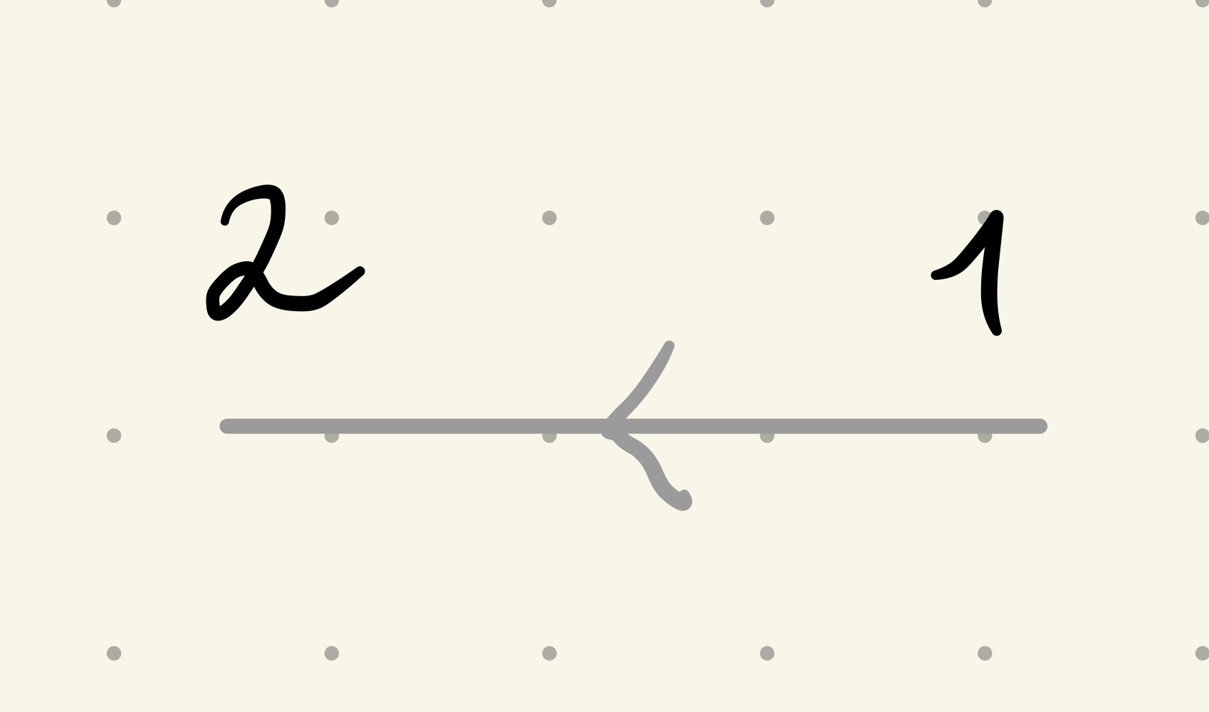
Propagator¶

The fully interacting one-particle propagator (or Green’s function) is the two-point correlation function defined as

\begin{align} G_{21} = -\langle c_2 \bar{c}_1 \rangle = - \frac{1}{Z} \int \mathcal{D}[\bar{c}, c] c_2 \bar{c}_1 e^{-S} \, . \end{align}

(2)

where (imaginary) time-ordering is implied. It is represented diagrammatically as

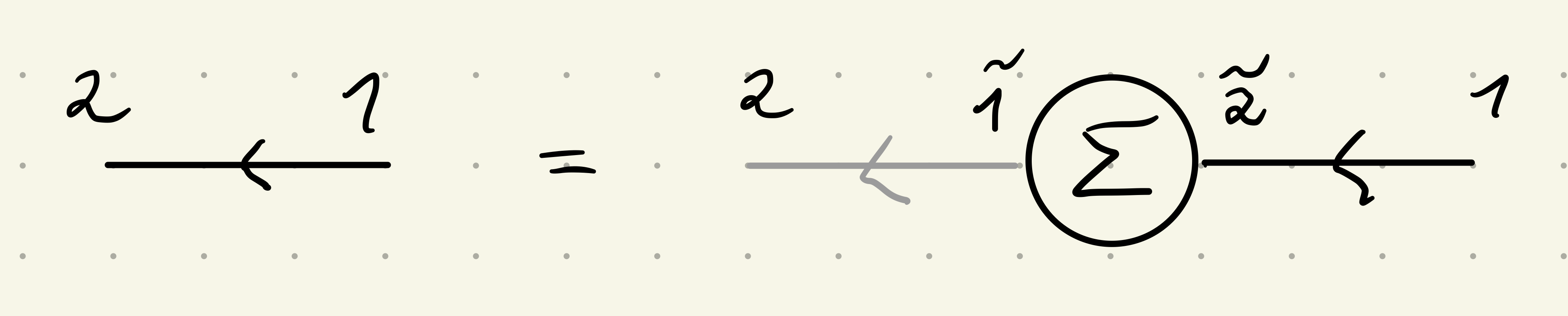
Self-energy¶

The main two-point quantity to compute in many-body theory is the one-particle irreducible two-point vertex, also called self-energy $\Sigma$ . It renormalizes single-particle properties and is formally defined via the Dyson equation,

\begin{align} G_{21} = G_{0,21} + G_{0,2\tilde{1}} \Sigma_{\tilde{1}\tilde{2}} G_{\tilde{2}1} \quad \Leftrightarrow \quad G^{-1}_{12} = (G_0)^{-1}_{12} - \Sigma_{12} \, , \end{align}

(3)

which is represented diagrammatically as

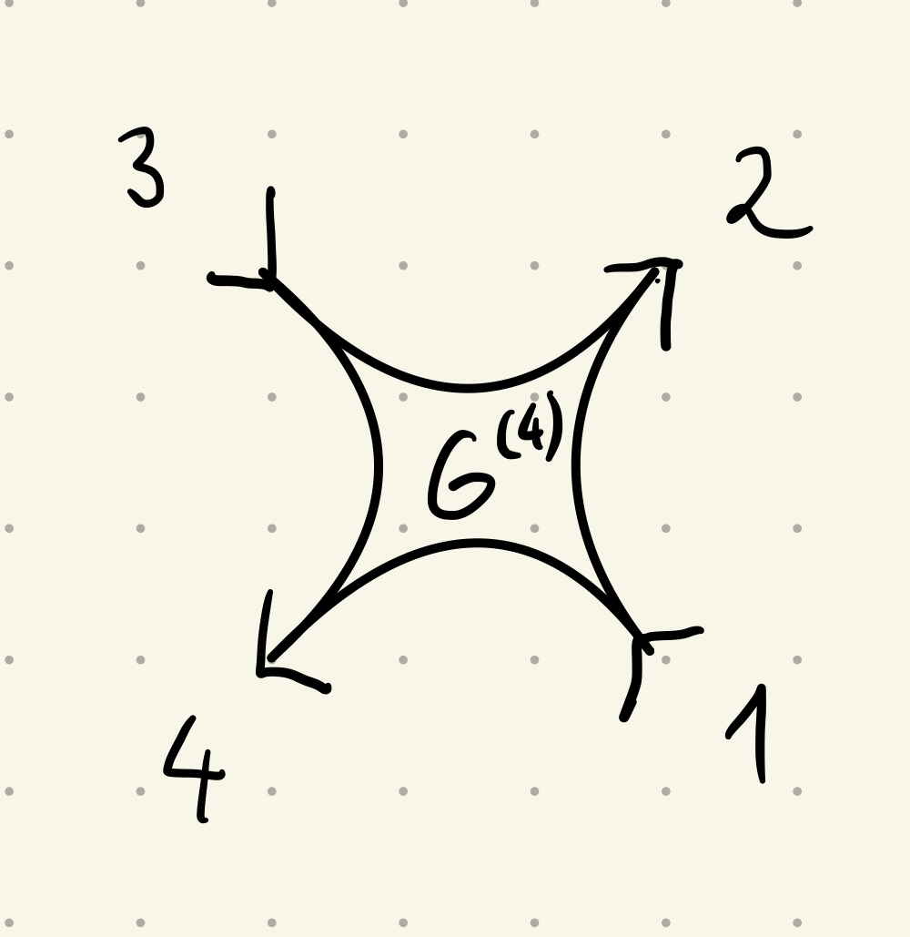
Four-point correlation function¶

The four-point correlation function is defined as

\begin{align} G^{(4)}_{4321} = \langle c_4 c_2 \bar{c}_3 \bar{c}_1 \rangle = \frac{1}{Z} \int \mathcal{D}[\bar{c}, c] c_4 c_2 \bar{c}_3 \bar{c}_1 e^{-S} \, , \end{align}

(4)

and represented diagrammatically by the flying squirrel diagram (credit: Marcel Gievers),

Note that in general, the order of multi-indices in correlation functions (such as $G$ and $G^{(4)}$ ) is reversed compared to that in vertex functions (such as $\Sigma$ and $F$ ).

Note

Some papers define the four-point correlation function with a different ordering of the operators as

\begin{align} \tilde{G}^{(4)}_{1234} = \langle c_1 \bar{c}_2 c_3 \bar{c}_4 \rangle \, , \end{align}

(5)

We can make contact with that convention by relabeling the indices in our definition of $G^{(4)}$ as

\begin{align} G^{(4)}_{1234} = \langle c_1 c_3 \bar{c}_2 \bar{c}_4 \rangle = \zeta \langle c_1 \bar{c}_2 c_3 \bar{c}_4 \rangle\, . \end{align}

(6)

Here, the factor $\zeta = -1$ for fermions and $\zeta = +1$ for bosons arises from exchanging the operators $c_3$ and $\bar{c}_2$ . For fermions, this sign factor leads to a global minus sign in all diagrammatic expressions involving four-point correlation function (including vertices!) compared to the convention used here.

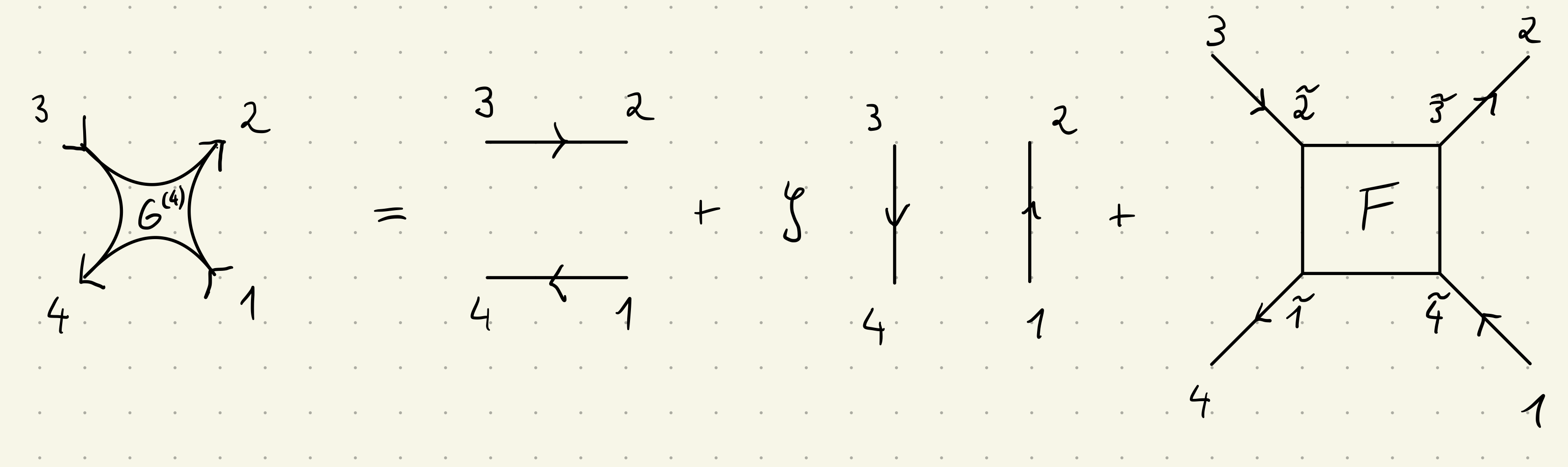
We can write down the tree expansion for the four-point function as

\begin{align} G^{(4)}_{4321} = G_{41} G_{23} + \zeta G_{43} G_{21} + G_{4\tilde{1}} G_{2\tilde{3}} F_{\tilde{1}\tilde{2}\tilde{3}\tilde{4}} G_{\tilde{2}3} G_{\tilde{4}1}\,. \end{align}

(7)

The third term, $G^{(4)}_{c,4321} = G_{4\tilde{1}} G_{2\tilde{3}} F_{\tilde{1}\tilde{2}\tilde{3}\tilde{4}} G_{\tilde{2}3} G_{\tilde{4}1}$ is also called the connected four point correlator. This expression defines the full four-point vertex $F$ .

Note on index ordering

It may look odd at first to write the indices in reverse order for the propagator and the four-point function. Indeed, one could have written $G^{(4)}_{1234} = \langle c_1 c_3 \overline{c}_2 \overline{c}_4 \rangle$ and $G_{12} = - \langle c_1 \overline{c}_2 \rangle$ , which just would have been a relabeling of indices. However, our notation has the advantage that odd indices always correspond to creation operators $\overline{c}$ and even indices to annihilation operators $c$ in the correlation functions and the action.

This structure is (almost) preserved when connecting vertices via propagator lines in diagrammatic expressions, as can already be seen in second order perturbation theory. The only exception is the $pp$ channel, where there has to be one connection with the swapped labeling.

Note that, as a consequence of this convention, the order of indices in the self-energy $\Sigma$ and vertex $F$ is reversed compared to that in the propagator $G$ and four-point function $G^{(4)}$ .