All diagrams contributing to the connected four-point correlator (or, equivalently, the four-point vertex) can be classified with respect to the property of two-particle reducibility. A diagram is called two-particle reducible if it can be separated into two parts by cutting a pair of internal propagator lines. Otherwise, it is called two-particle irreducible . The set of all two-particle reducible diagrams can furthermore be uniquely decomposed into three topologically distinct two-particle channels : the particle-particle (p p pp pp p h ph p h p h ‾ \overline{ph} p h
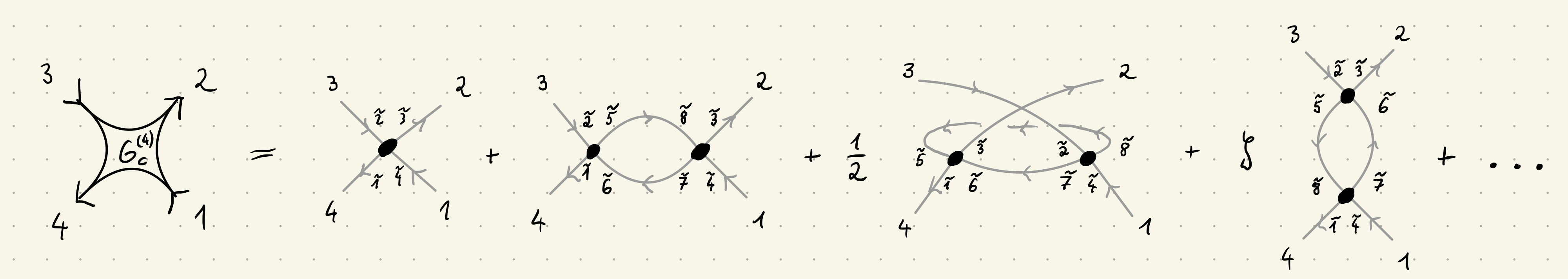
Second-order perturbation theory ¶ The three channels are apparent already at the level of the second-order diagrams in perturbation theory. For the connected four-point correlator, we obtain three contributions beyond the first-order diagram:
G c , 4321 ( 4 ) = G 0 , 4 1 ~ G 0 , 2 ~ 3 F 0 , 1 ~ 2 ~ 3 ~ 4 ~ G 0 , 2 3 ~ G 0 , 4 ~ 1 = + G 0 , 4 1 ~ G 0 , 2 ~ 3 F 0 , 1 ~ 2 ~ 5 ~ 6 ~ G 0 , 6 ~ 7 ~ G 0 , 8 ~ 5 ~ F 0 , 7 ~ 8 ~ 3 ~ 4 ~ G 0 , 2 3 ~ G 0 , 4 ~ 1 ( p h ‾ channel) = + 1 2 G 0 , 4 1 ~ G 0 , 2 ~ 3 F 0 , 1 ~ 5 ~ 3 ~ 6 ~ G 0 , 6 ~ 7 ~ G 0 , 5 ~ 8 ~ F 0 , 7 ~ 2 ~ 8 ~ 4 ~ G 0 , 2 3 ~ G 0 , 4 ~ 1 ( p p channel) = + ζ G 0 , 2 ~ 3 G 0 , 2 3 ~ F 0 , 5 ~ 2 ~ 3 ~ 6 ~ G 0 , 6 ~ 7 ~ G 0 , 8 ~ 5 ~ F 0 , 1 ~ 8 ~ 7 ~ 4 ~ G 0 , 4 1 ~ G 0 , 4 ~ 1 ( p h channel) = + O ( F 0 3 ) . \begin{align}
G^{(4)}_{c,4321} &= G_{0,4\tilde{1}} G_{0,\tilde{2}3} F_{0,\tilde{1}\tilde{2}\tilde{3}\tilde{4}} G_{0,2\tilde{3}} G_{0,\tilde{4}1} \\
&\phantom{=} + G_{0,4\tilde{1}} G_{0,\tilde{2}3} F_{0,\tilde{1}\tilde{2}\tilde{5}\tilde{6}} G_{0,\tilde{6}\tilde{7}} G_{0,\tilde{8}\tilde{5}} F_{0,\tilde{7}\tilde{8}\tilde{3}\tilde{4}} G_{0,2\tilde{3}} G_{0,\tilde{4}1} \quad \text{($\overline{ph}$ channel)} \\
&\phantom{=} + \frac{1}{2} G_{0,4\tilde{1}} G_{0,\tilde{2}3} F_{0,\tilde{1}\tilde{5}\tilde{3}\tilde{6}} G_{0,\tilde{6}\tilde{7}} G_{0,\tilde{5}\tilde{8}} F_{0,\tilde{7}\tilde{2}\tilde{8}\tilde{4}} G_{0,2\tilde{3}} G_{0,\tilde{4}1} \quad \text{($pp$ channel)} \\
&\phantom{=} + \zeta G_{0,\tilde{2} 3} G_{0,2\tilde{3}} F_{0,\tilde{5}\tilde{2}\tilde{3}\tilde{6}} G_{0,\tilde{6}\tilde{7}} G_{0,\tilde{8}\tilde{5}} F_{0,\tilde{1}\tilde{8}\tilde{7}\tilde{4}} G_{0,4\tilde{1}} G_{0,\tilde{4}1} \quad \text{($ph$ channel)} \\
&\phantom{=} + \mathcal{O}(F_0^3)\, .
\end{align} G c , 4321 ( 4 ) = G 0 , 4 1 ~ G 0 , 2 ~ 3 F 0 , 1 ~ 2 ~ 3 ~ 4 ~ G 0 , 2 3 ~ G 0 , 4 ~ 1 = + G 0 , 4 1 ~ G 0 , 2 ~ 3 F 0 , 1 ~ 2 ~ 5 ~ 6 ~ G 0 , 6 ~ 7 ~ G 0 , 8 ~ 5 ~ F 0 , 7 ~ 8 ~ 3 ~ 4 ~ G 0 , 2 3 ~ G 0 , 4 ~ 1 ( p h channel) = + 2 1 G 0 , 4 1 ~ G 0 , 2 ~ 3 F 0 , 1 ~ 5 ~ 3 ~ 6 ~ G 0 , 6 ~ 7 ~ G 0 , 5 ~ 8 ~ F 0 , 7 ~ 2 ~ 8 ~ 4 ~ G 0 , 2 3 ~ G 0 , 4 ~ 1 ( pp channel) = + ζ G 0 , 2 ~ 3 G 0 , 2 3 ~ F 0 , 5 ~ 2 ~ 3 ~ 6 ~ G 0 , 6 ~ 7 ~ G 0 , 8 ~ 5 ~ F 0 , 1 ~ 8 ~ 7 ~ 4 ~ G 0 , 4 1 ~ G 0 , 4 ~ 1 ( p h channel) = + O ( F 0 3 ) . Derive this expression, including all Wick contractions and sign factors. See Jan’s handwritten notes for reference.
Also, since there is some ambiguity in the literature regarding the labeling of the two particle-hole channels, we should clarify our conventions here. Write up Fabian’s explanation in an accessible way.
Note that the connected four-point correlator is crossing symmetric as well, i.e., it is invariant under the exchange of any two external legs (up to a sign factor ζ \zeta ζ p h ‾ \overline{ph} p h p h ph p h p p pp pp
Exchanging the two outgoing legs 2 ↔ 4 2\leftrightarrow 4 2 ↔ 4 p h ph p h 1 ~ → 3 ~ \tilde{1} \rightarrow \tilde{3} 1 ~ → 3 ~
ζ G 0 , 2 ~ 3 G 0 , 4 3 ~ F 0 , 5 ~ 2 ~ 3 ~ 6 ~ G 0 , 6 ~ 7 ~ G 0 , 8 ~ 5 ~ F 0 , 1 ~ 8 ~ 7 ~ 4 ~ G 0 , 2 1 ~ G 0 , 4 ~ 1 = ζ G 0 , 2 ~ 3 G 0 , 4 1 ~ F 0 , 5 ~ 2 ~ 1 ~ 6 ~ G 0 , 6 ~ 7 ~ G 0 , 8 ~ 5 ~ F 0 , 3 ~ 8 ~ 7 ~ 4 ~ G 0 , 2 3 ~ G 0 , 4 ~ 1 = ζ G 0 , 2 ~ 3 G 0 , 4 1 ~ ( ζ F 0 , 1 ~ 2 ~ 5 ~ 6 ~ ) G 0 , 6 ~ 7 ~ G 0 , 8 ~ 5 ~ ( ζ F 0 , 7 ~ 8 ~ 3 ~ 4 ~ ) G 0 , 2 3 ~ G 0 , 4 ~ 1 = ζ G 0 , 4 1 ~ G 0 , 2 ~ 3 F 0 , 1 ~ 2 ~ 5 ~ 6 ~ G 0 , 6 ~ 7 ~ G 0 , 8 ~ 5 ~ F 0 , 7 ~ 8 ~ 3 ~ 4 ~ G 0 , 2 3 ~ G 0 , 4 ~ 1 , \begin{align}
&\zeta G_{0,\tilde{2} 3} G_{0,4\tilde{3}} F_{0,\tilde{5}\tilde{2}\tilde{3}\tilde{6}} G_{0,\tilde{6}\tilde{7}} G_{0,\tilde{8}\tilde{5}} F_{0,\tilde{1}\tilde{8}\tilde{7}\tilde{4}} G_{0,2\tilde{1}} G_{0,\tilde{4}1} \\
&= \zeta G_{0,\tilde{2} 3} G_{0,4\tilde{1}} F_{0,\tilde{5}\tilde{2}\tilde{1}\tilde{6}} G_{0,\tilde{6}\tilde{7}} G_{0,\tilde{8}\tilde{5}} F_{0,\tilde{3}\tilde{8}\tilde{7}\tilde{4}} G_{0,2\tilde{3}} G_{0,\tilde{4}1} \\
&= \zeta G_{0,\tilde{2} 3} G_{0,4\tilde{1}} (\zeta F_{0,\tilde{1}\tilde{2}\tilde{5}\tilde{6}}) G_{0,\tilde{6}\tilde{7}} G_{0,\tilde{8}\tilde{5}} (\zeta F_{0,\tilde{7}\tilde{8}\tilde{3}\tilde{4}}) G_{0,2\tilde{3}} G_{0,\tilde{4}1} \\
&= \zeta G_{0,4\tilde{1}} G_{0,\tilde{2} 3} F_{0,\tilde{1}\tilde{2}\tilde{5}\tilde{6}} G_{0,\tilde{6}\tilde{7}} G_{0,\tilde{8}\tilde{5}} F_{0,\tilde{7}\tilde{8}\tilde{3}\tilde{4}} G_{0,2\tilde{3}} G_{0,\tilde{4}1}\, ,
\end{align} ζ G 0 , 2 ~ 3 G 0 , 4 3 ~ F 0 , 5 ~ 2 ~ 3 ~ 6 ~ G 0 , 6 ~ 7 ~ G 0 , 8 ~ 5 ~ F 0 , 1 ~ 8 ~ 7 ~ 4 ~ G 0 , 2 1 ~ G 0 , 4 ~ 1 = ζ G 0 , 2 ~ 3 G 0 , 4 1 ~ F 0 , 5 ~ 2 ~ 1 ~ 6 ~ G 0 , 6 ~ 7 ~ G 0 , 8 ~ 5 ~ F 0 , 3 ~ 8 ~ 7 ~ 4 ~ G 0 , 2 3 ~ G 0 , 4 ~ 1 = ζ G 0 , 2 ~ 3 G 0 , 4 1 ~ ( ζ F 0 , 1 ~ 2 ~ 5 ~ 6 ~ ) G 0 , 6 ~ 7 ~ G 0 , 8 ~ 5 ~ ( ζ F 0 , 7 ~ 8 ~ 3 ~ 4 ~ ) G 0 , 2 3 ~ G 0 , 4 ~ 1 = ζ G 0 , 4 1 ~ G 0 , 2 ~ 3 F 0 , 1 ~ 2 ~ 5 ~ 6 ~ G 0 , 6 ~ 7 ~ G 0 , 8 ~ 5 ~ F 0 , 7 ~ 8 ~ 3 ~ 4 ~ G 0 , 2 3 ~ G 0 , 4 ~ 1 , which is indeed ζ \zeta ζ p h ‾ \overline{ph} p h p p pp pp 2 ↔ 4 2\leftrightarrow 4 2 ↔ 4 1 ~ → 3 ~ \tilde{1} \rightarrow \tilde{3} 1 ~ → 3 ~
1 2 G 0 , 2 1 ~ G 0 , 2 ~ 3 F 0 , 1 ~ 5 ~ 3 ~ 6 ~ G 0 , 6 ~ 7 ~ G 0 , 5 ~ 8 ~ F 0 , 7 ~ 2 ~ 8 ~ 4 ~ G 0 , 4 3 ~ G 0 , 4 ~ 1 = 1 2 G 0 , 2 3 ~ G 0 , 2 ~ 3 F 0 , 3 ~ 5 ~ 1 ~ 6 ~ G 0 , 6 ~ 7 ~ G 0 , 5 ~ 8 ~ F 0 , 7 ~ 2 ~ 8 ~ 4 ~ G 0 , 4 1 ~ G 0 , 4 ~ 1 = 1 2 G 0 , 4 1 ~ G 0 , 2 ~ 3 ( ζ F 0 , 1 ~ 5 ~ 3 ~ 6 ~ ) G 0 , 6 ~ 7 ~ G 0 , 5 ~ 8 ~ F 0 , 7 ~ 2 ~ 8 ~ 4 ~ G 0 , 2 3 ~ G 0 , 4 ~ 1 , \begin{align}
&\frac{1}{2} G_{0,2\tilde{1}} G_{0,\tilde{2}3} F_{0,\tilde{1}\tilde{5}\tilde{3}\tilde{6}} G_{0,\tilde{6}\tilde{7}} G_{0,\tilde{5}\tilde{8}} F_{0,\tilde{7}\tilde{2}\tilde{8}\tilde{4}} G_{0,4\tilde{3}} G_{0,\tilde{4}1} \\
&= \frac{1}{2} G_{0,2\tilde{3}} G_{0,\tilde{2}3} F_{0,\tilde{3}\tilde{5}\tilde{1}\tilde{6}} G_{0,\tilde{6}\tilde{7}} G_{0,\tilde{5}\tilde{8}} F_{0,\tilde{7}\tilde{2}\tilde{8}\tilde{4}} G_{0,4\tilde{1}} G_{0,\tilde{4}1} \\
&= \frac{1}{2} G_{0,4\tilde{1}} G_{0,\tilde{2}3} (\zeta F_{0,\tilde{1}\tilde{5}\tilde{3}\tilde{6}}) G_{0,\tilde{6}\tilde{7}} G_{0,\tilde{5}\tilde{8}} F_{0,\tilde{7}\tilde{2}\tilde{8}\tilde{4}} G_{0,2\tilde{3}} G_{0,\tilde{4}1}\, ,
\end{align} 2 1 G 0 , 2 1 ~ G 0 , 2 ~ 3 F 0 , 1 ~ 5 ~ 3 ~ 6 ~ G 0 , 6 ~ 7 ~ G 0 , 5 ~ 8 ~ F 0 , 7 ~ 2 ~ 8 ~ 4 ~ G 0 , 4 3 ~ G 0 , 4 ~ 1 = 2 1 G 0 , 2 3 ~ G 0 , 2 ~ 3 F 0 , 3 ~ 5 ~ 1 ~ 6 ~ G 0 , 6 ~ 7 ~ G 0 , 5 ~ 8 ~ F 0 , 7 ~ 2 ~ 8 ~ 4 ~ G 0 , 4 1 ~ G 0 , 4 ~ 1 = 2 1 G 0 , 4 1 ~ G 0 , 2 ~ 3 ( ζ F 0 , 1 ~ 5 ~ 3 ~ 6 ~ ) G 0 , 6 ~ 7 ~ G 0 , 5 ~ 8 ~ F 0 , 7 ~ 2 ~ 8 ~ 4 ~ G 0 , 2 3 ~ G 0 , 4 ~ 1 , which is indeed equal to the ζ \zeta ζ p p pp pp
From this point on, it is convenient to work directly with the four-point vertex F F F G c ( 4 ) G^{(4)}_c G c ( 4 )
F 1234 = F 0 , 1234 + F 0 , 1256 G 0 , 67 G 0 , 85 F 0 , 7834 ( p h ‾ channel) + 1 2 F 0 , 1536 G 0 , 67 G 0 , 58 F 0 , 7284 ( p p channel) + ζ F 0 , 5236 G 0 , 67 G 0 , 85 F 0 , 1874 ( p h channel) + O ( F 0 3 ) . \begin{align}
F_{1234} = F_{0,1234} &+ F_{0,1256} G_{0,67} G_{0,85} F_{0,7834} \quad \text{($\overline{ph}$ channel)} \\
&+ \frac{1}{2} F_{0,1536} G_{0,67} G_{0,58} F_{0,7284} \quad \text{($pp$ channel)}\\
&+ \zeta F_{0,5236} G_{0,67} G_{0,85} F_{0,1874} \quad \text{($ph$ channel)}\\
&+ \mathcal{O}(F_0^3)\, .
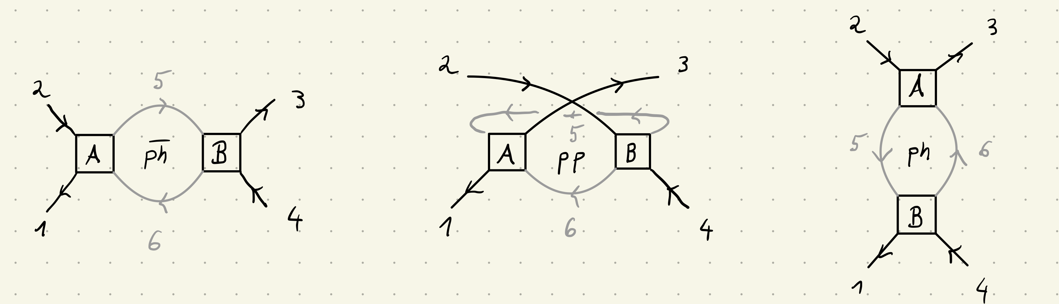
\end{align} F 1234 = F 0 , 1234 + F 0 , 1256 G 0 , 67 G 0 , 85 F 0 , 7834 ( p h channel) + 2 1 F 0 , 1536 G 0 , 67 G 0 , 58 F 0 , 7284 ( pp channel) + ζ F 0 , 5236 G 0 , 67 G 0 , 85 F 0 , 1874 ( p h channel) + O ( F 0 3 ) . Connectors and identity operators ¶ For ease of notation, it is useful to define a connector ∘ to denote summation over all indices in each two-particle channel as
[ A ∘ B ] 1234 p h ‾ = A 1256 B 6534 [ A ∘ B ] 1234 p p = A 1536 B 6254 [ A ∘ B ] 1234 p h = A 5236 B 1564 . \begin{align}
[A\circ B]^{\overline{ph}}_{1234} &= A_{1256} B_{6534} \\
[A\circ B]^{pp}_{1234} &= A_{1536} B_{6254} \\
[A\circ B]^{ph}_{1234} &= A_{5236} B_{1564}\, .
\end{align} [ A ∘ B ] 1234 p h [ A ∘ B ] 1234 pp [ A ∘ B ] 1234 p h = A 1256 B 6534 = A 1536 B 6254 = A 5236 B 1564 . For later use, it is convenient to also define the channel-specific identity operators 1 r \mathbb{1}^r 1 r A = 1 r ∘ A = A ∘ 1 r A = \mathbb{1}^r \circ A = A \circ \mathbb{1}^r A = 1 r ∘ A = A ∘ 1 r r ∈ { p h ‾ , p p , p h } r\in\{\overline{ph}, pp, ph\} r ∈ { p h , pp , p h }
1 1234 p h ‾ = δ 14 δ 23 = 1 1234 p p 1 1234 p h = δ 12 δ 34 . \begin{align}
\mathbb{1}^{\overline{ph}}_{1234} &= \delta_{14} \delta_{23} = \mathbb{1}^{pp}_{1234} \\
\mathbb{1}^{ph}_{1234} &= \delta_{12} \delta_{34} \, .
\end{align} 1 1234 p h 1 1234 p h = δ 14 δ 23 = 1 1234 pp = δ 12 δ 34 . Demonstrating that the identity operators defined this way work as intended is straightforward but somewhat tedious. Here, we explicitly write out all indices for each channel to show that the definitions are correct.
[ A ∘ 1 p h ‾ ] 1234 = A 1256 1 6534 p h ‾ = A 1256 δ 64 δ 53 = A 1234 [ 1 p h ‾ ∘ A ] 1234 = 1 1256 p h ‾ A 6534 = δ 16 δ 25 A 6534 = A 1234 [ A ∘ 1 p p ] 1234 = A 1536 1 6254 p p = A 1536 δ 64 δ 25 = A 1234 [ 1 p p ∘ A ] 1234 = 1 1536 p p A 6254 = δ 61 δ 53 A 6254 = A 1234 [ A ∘ 1 p h ] 1234 = A 5236 1 1564 p h = A 5236 δ 15 δ 64 = A 1234 [ 1 p h ∘ A ] 1234 = 1 5236 p h A 1564 = δ 52 δ 36 A 1564 = A 1234 . \begin{align}
[A \circ \mathbb{1}^{\overline{ph}}]_{1234} &= A_{1256} \mathbb{1}^{\overline{ph}}_{6534} = A_{1256} \delta_{64} \delta_{53} = A_{1234} \\
[\mathbb{1}^{\overline{ph}} \circ A]_{1234} &= \mathbb{1}^{\overline{ph}}_{1256} A_{6534} = \delta_{16} \delta_{25} A_{6534} = A_{1234} \\ \\
[A \circ \mathbb{1}^{pp}]_{1234} &= A_{1536} \mathbb{1}^{pp}_{6254} = A_{1536} \delta_{64} \delta_{25} = A_{1234} \\
[\mathbb{1}^{pp} \circ A]_{1234} &= \mathbb{1}^{pp}_{1536} A_{6254} = \delta_{61} \delta_{53} A_{6254} = A_{1234} \\ \\
[A \circ \mathbb{1}^{ph}]_{1234} &= A_{5236} \mathbb{1}^{ph}_{1564} = A_{5236} \delta_{15} \delta_{64} = A_{1234} \\
[\mathbb{1}^{ph} \circ A]_{1234} &= \mathbb{1}^{ph}_{5236} A_{1564} = \delta_{52} \delta_{36} A_{1564} = A_{1234} \, .
\end{align} [ A ∘ 1 p h ] 1234 [ 1 p h ∘ A ] 1234 [ A ∘ 1 pp ] 1234 [ 1 pp ∘ A ] 1234 [ A ∘ 1 p h ] 1234 [ 1 p h ∘ A ] 1234 = A 1256 1 6534 p h = A 1256 δ 64 δ 53 = A 1234 = 1 1256 p h A 6534 = δ 16 δ 25 A 6534 = A 1234 = A 1536 1 6254 pp = A 1536 δ 64 δ 25 = A 1234 = 1 1536 pp A 6254 = δ 61 δ 53 A 6254 = A 1234 = A 5236 1 1564 p h = A 5236 δ 15 δ 64 = A 1234 = 1 5236 p h A 1564 = δ 52 δ 36 A 1564 = A 1234 . Indeed, the identity operators have the right properties. ✓ \checkmark ✓
These identity operators can also be used to define the inverse of a four-point quantity A A A
[ A − 1 ] 1234 r such that [ A − 1 ] r ∘ A = A ∘ [ A − 1 ] r = 1 r . \begin{align}
[A^{-1}]^r_{1234} \quad \text{such that} \quad [A^{-1}]^r \circ A = A \circ [A^{-1}]^r = \mathbb{1}^r \, .
\end{align} [ A − 1 ] 1234 r such that [ A − 1 ] r ∘ A = A ∘ [ A − 1 ] r = 1 r . Bare and dressed bubbles ¶ We furthermore define the bare bubble as
[ χ 0 0 ] 4321 = G 0 , 41 G 0 , 23 . \begin{align}
[\chi_0^0]_{4321} = G_{0,41} G_{0,23} \, .
\end{align} [ χ 0 0 ] 4321 = G 0 , 41 G 0 , 23 . The notation is not optimal here. The subscript “0” shall indicate that this object is distinct from a susceptibility (in fact, it is effectively the bubble term without vertex corrections). The superscript “0” is meant to indicate that this is the bare version of the bubble. However, having two zeros in the same symbol is confusing. We should think about better notation.
This object is used to define the bare bubble in each two-particle channel as
[ χ 0 0 ] 4321 p h ‾ = [ χ 0 0 ] 4321 [ χ 0 0 ] 4321 p p = 1 2 [ χ 0 0 ] 4321 [ χ 0 0 ] 4321 p h = ζ [ χ 0 0 ] 2341 . \begin{align}
[\chi_0^0]^{\overline{ph}}_{4321} &= [\chi_0^0]_{4321} \\
[\chi_0^0]^{pp}_{4321} &= \frac{1}{2} [\chi_0^0]_{4321} \\
[\chi_0^0]^{ph}_{4321} &= \zeta [\chi_0^0]_{2341} \, .
\end{align} [ χ 0 0 ] 4321 p h [ χ 0 0 ] 4321 pp [ χ 0 0 ] 4321 p h = [ χ 0 0 ] 4321 = 2 1 [ χ 0 0 ] 4321 = ζ [ χ 0 0 ] 2341 . With these definitions, we have a unified notation for the three two-particle channels, and we can write the second-order perturbation theory expression for the four-point vertex as
F 1234 = F 0 , 1234 + ∑ r ∈ { p h ‾ , p p , p h } ( F 0 ∘ [ χ 0 0 ] r ∘ F 0 ) 1234 + O ( F 0 3 ) , \begin{align}
F_{1234} = F_{0,1234} + \sum_{r\in\{\overline{ph}, pp, ph\}}(F_0 \circ [\chi_0^0]^r \circ F_0)_{1234} + \mathcal{O}(F_0^3)\, ,
\end{align} F 1234 = F 0 , 1234 + r ∈ { p h , pp , p h } ∑ ( F 0 ∘ [ χ 0 0 ] r ∘ F 0 ) 1234 + O ( F 0 3 ) , or simply
F = F 0 + ∑ r F 0 ∘ [ χ 0 0 ] r ∘ F 0 + O ( F 0 3 ) . \begin{align}
F = F_0 + \sum_{r} F_0 \circ [\chi_0^0]^r \circ F_0 + \mathcal{O}(F_0^3)\, .
\end{align} F = F 0 + r ∑ F 0 ∘ [ χ 0 0 ] r ∘ F 0 + O ( F 0 3 ) . With the definitions of the channel-specific connectors ∘ and the bare bubbles [ χ 0 0 ] r [\chi_0^0]^r [ χ 0 0 ] r
p h ‾ : [ F 0 ∘ [ χ 0 0 ] p h ‾ ∘ F 0 ] 1234 = F 0 , 1256 [ [ χ 0 0 ] p h ‾ ∘ F ] 6534 = F 0 , 1256 [ χ 0 0 ] 6587 p h ‾ F 0 , 7834 = F 0 , 1256 [ χ 0 0 ] 6587 F 0 , 7834 = F 0 , 1256 G 0 , 67 G 0 , 85 F 0 , 7834 p p : [ F 0 ∘ [ χ 0 0 ] p p ∘ F 0 ] 1234 = F 0 , 1536 [ [ χ 0 0 ] p p ∘ F ] 6254 = F 0 , 1536 [ χ 0 0 ] 6857 p p F 0 , 7284 = 1 2 F 0 , 1536 [ χ 0 0 ] 6857 F 0 , 7284 = 1 2 F 0 , 1536 G 0 , 67 G 0 , 58 F 0 , 7284 p h : [ F 0 ∘ [ χ 0 0 ] p h ∘ F 0 ] 1234 = F 0 , 5236 [ [ χ 0 0 ] p h ∘ F ] 1564 = F 0 , 5236 [ χ 0 0 ] 8567 p h F 0 , 1874 = ζ F 0 , 5236 [ χ 0 0 ] 6587 F 0 , 1874 = ζ F 0 , 5236 G 0 , 67 G 0 , 85 F 0 , 1874 . \begin{align}
\text{$\overline{ph}$:}\quad [F_0 \circ [\chi_0^0]^{\overline{ph}} \circ F_0]_{1234} &= F_{0,1256} [[\chi_0^0]^{\overline{ph}} \circ F]_{6534} = F_{0,1256} [\chi_0^0]^{\overline{ph}}_{6587} F_{0,7834} \\
&= F_{0,1256} [\chi_0^0]_{6587} F_{0,7834} = F_{0,1256} G_{0,67} G_{0,85} F_{0,7834} \\ \\
\text{$pp$:}\quad [F_0 \circ [\chi_0^0]^{pp} \circ F_0]_{1234} &= F_{0,1536} [[\chi_0^0]^{pp} \circ F]_{6254} = F_{0,1536} [\chi_0^0]^{pp}_{6857} F_{0,7284} \\
&= \frac{1}{2} F_{0,1536} [\chi_0^0]_{6857} F_{0,7284} = \frac{1}{2} F_{0,1536} G_{0,67} G_{0,58} F_{0,7284} \\ \\
\text{$ph$:}\quad [F_0 \circ [\chi_0^0]^{ph} \circ F_0]_{1234} &= F_{0,5236} [[\chi_0^0]^{ph} \circ F]_{1564} = F_{0,5236} [\chi_0^0]^{ph}_{8567} F_{0,1874} \\
&= \zeta F_{0,5236} [\chi_0^0]_{6587} F_{0,1874} = \zeta F_{0,5236} G_{0,67} G_{0,85} F_{0,1874} \, .
\end{align} p h : [ F 0 ∘ [ χ 0 0 ] p h ∘ F 0 ] 1234 pp : [ F 0 ∘ [ χ 0 0 ] pp ∘ F 0 ] 1234 p h : [ F 0 ∘ [ χ 0 0 ] p h ∘ F 0 ] 1234 = F 0 , 1256 [[ χ 0 0 ] p h ∘ F ] 6534 = F 0 , 1256 [ χ 0 0 ] 6587 p h F 0 , 7834 = F 0 , 1256 [ χ 0 0 ] 6587 F 0 , 7834 = F 0 , 1256 G 0 , 67 G 0 , 85 F 0 , 7834 = F 0 , 1536 [[ χ 0 0 ] pp ∘ F ] 6254 = F 0 , 1536 [ χ 0 0 ] 6857 pp F 0 , 7284 = 2 1 F 0 , 1536 [ χ 0 0 ] 6857 F 0 , 7284 = 2 1 F 0 , 1536 G 0 , 67 G 0 , 58 F 0 , 7284 = F 0 , 5236 [[ χ 0 0 ] p h ∘ F ] 1564 = F 0 , 5236 [ χ 0 0 ] 8567 p h F 0 , 1874 = ζ F 0 , 5236 [ χ 0 0 ] 6587 F 0 , 1874 = ζ F 0 , 5236 G 0 , 67 G 0 , 85 F 0 , 1874 . These are indeed the correct expressions. ✓ \checkmark ✓
For later use, we also define the dressed bubble , sometimes also called Lindhard function , in the same manner as the bare bubble, but with full propagators instead of bare ones:
[ χ 0 ] 4321 = G 41 G 23 \begin{align}
[\chi_0]_{4321} = G_{41} G_{23} \,
\end{align} [ χ 0 ] 4321 = G 41 G 23 and
[ χ 0 ] 4321 p h ‾ = [ χ 0 ] 4321 [ χ 0 ] 4321 p p = 1 2 [ χ 0 ] 4321 [ χ 0 ] 4321 p h = ζ [ χ 0 ] 2341 . \begin{align}
[\chi_0]^{\overline{ph}}_{4321} &= [\chi_0]_{4321} \\
[\chi_0]^{pp}_{4321} &= \frac{1}{2} [\chi_0]_{4321} \\
[\chi_0]^{ph}_{4321} &= \zeta [\chi_0]_{2341} \, .
\end{align} [ χ 0 ] 4321 p h [ χ 0 ] 4321 pp [ χ 0 ] 4321 p h = [ χ 0 ] 4321 = 2 1 [ χ 0 ] 4321 = ζ [ χ 0 ] 2341 . Note on possible confusion regarding p h ↔ p h ‾ ph \leftrightarrow \overline{ph} p h ↔ p h ¶ There is some ambiguity in the literature regarding the labeling of the two particle-hole channels. This confusion arises, because, for general models, in which both two fermion lines enter and exit each vertex, there is no fundamental difference between the two particle-hole channels, since they are related by crossing symmetry: Swapping the pair of entering or exiting legs, respectively, transforms one channel into the other and generates a minus sign (for fermions).
In fact, one can also generate a minus sign in the p p pp pp χ 0 p p \chi_0^{pp} χ 0 pp F F F − F -F − F
The distinction between the two channels only becomes unambiguous, when spin indices are specified (for details, see the section on spin parametrizations ). That is because with the label p h ph p h σ \sigma σ ν \nu ν σ ′ \sigma' σ ′ ν ′ \nu' ν ′ ω = 0 \omega=0 ω = 0 σ \sigma σ σ ′ \sigma' σ ′ p h ph p h
Attaching σ \sigma σ σ ′ \sigma' σ ′ p h ph p h G σ ′ σ σ σ ′ = ⟨ c σ ′ c σ c ‾ σ c ‾ σ ′ ⟩ = ζ 4 ⟨ c ‾ σ ′ c σ ′ c ‾ σ c σ ⟩ = ⟨ n σ ′ n σ ⟩ G_{\sigma'\sigma\sigma\sigma'} = \langle c_{\sigma'} c_{\sigma} \overline{c}_{\sigma} \overline{c}_{\sigma'} \rangle = \zeta^4 \langle \overline{c}_{\sigma'} c_{\sigma'} \overline{c}_{\sigma} c_{\sigma} \rangle = \langle n_{\sigma'} n_\sigma \rangle G σ ′ σσ σ ′ = ⟨ c σ ′ c σ c σ c σ ′ ⟩ = ζ 4 ⟨ c σ ′ c σ ′ c σ c σ ⟩ = ⟨ n σ ′ n σ ⟩ σ \sigma σ ν \nu ν σ ′ \sigma' σ ′ ν ′ \nu' ν ′ basic quantities . This is precisely the density-density (or “charge”) correlator, which probes particle-hole excitations!
and has been also historically used, for example in large parts of the fRG literature (to do: Cite Honerkamp and mfRG papers), but also in multipoint-NRG (to do: cite those papers) and even in the Vienna community (see Fig. 1 in Wentzell et al. (2020)
In many papers from the Vienna community, including Rohringer et al. (2012) Rohringer et al. (2018) σ \sigma σ σ ′ \sigma' σ ′ p h ph p h ↑ ↓ \uparrow \downarrow ↑↓ spin parametrizations for more details.
It should be noted that this choice can be made consistent with the label p h ph p h four-point correlation function ). Then, attaching σ \sigma σ σ ′ \sigma' σ ′ G ~ σ σ σ ′ σ ′ = ⟨ c σ c ‾ σ c σ ′ c ‾ σ ′ ⟩ = ζ 2 ⟨ c ‾ σ c σ c ‾ σ ′ c σ ′ ⟩ = ⟨ n σ n σ ′ ⟩ \tilde{G}_{\sigma\sigma \sigma'\sigma'} = \langle c_{\sigma} \overline{c}_{\sigma} c_{\sigma'} \overline{c}_{\sigma'} \rangle = \zeta^2 \langle \overline{c}_{\sigma} c_{\sigma} \overline{c}_{\sigma'} c_{\sigma'} \rangle = \langle n_{\sigma} n_{\sigma'} \rangle G ~ σσ σ ′ σ ′ = ⟨ c σ c σ c σ ′ c σ ′ ⟩ = ζ 2 ⟨ c σ c σ c σ ′ c σ ′ ⟩ = ⟨ n σ n σ ′ ⟩
Thanks to Fabian Kugler for large parts of this explanation!
Wentzell, N., Li, G., Tagliavini, A., Taranto, C., Rohringer, G., Held, K., Toschi, A., & Andergassen, S. (2020). High-frequency asymptotics of the vertex function: Diagrammatic parametrization and algorithmic implementation. Physical Review B , 102 (8). 10.1103/physrevb.102.085106 Rohringer, G., Valli, A., & Toschi, A. (2012). Local electronic correlation at the two-particle level. Physical Review B , 86 (12). 10.1103/physrevb.86.125114 Rohringer, G., Hafermann, H., Toschi, A., Katanin, A. A., Antipov, A. E., Katsnelson, M. I., Lichtenstein, A. I., Rubtsov, A. N., & Held, K. (2018). Diagrammatic routes to nonlocal correlations beyond dynamical mean field theory. Reviews of Modern Physics , 90 (2). 10.1103/revmodphys.90.025003