Parquet theory - TwoParticleQFT

The concept of two-particle reducibility of certain diagrams, introduced in the section on two-particle channels, can be formalized further. In particular, it allows us to decompose the full two-particle vertex $F$ into four distinct different contributions. This decomposition is known as the parquet decomposition and forms the basis of parquet theory.

Parquet decomposition¶

As discussed previously, any given diagram is called two-particle reducible if it can be separated into two parts by cutting a pair of internal propagator lines, and there are three distinct channels in which this can happen: the particle-hole ( $ph$ ), the transverse particle-hole ( $\overline{ph}$ ), and the particle-particle ( $pp$ ) channel. A diagram that is not two-particle reducible in a given channel is called two-particle irreducible in that channel. Finally, a diagram that is not two-particle reducible in any of the three channels is called fully irreducible.

The sum of all two-particle diagrams reducible in channel $r \in \{\overline{ph}, pp, ph\}$ is denoted by $\Phi^r$ , while the sum of all fully irreducible diagrams is denoted by $\Lambda$ . Since these classes are distinct, the full vertex $F$ can be decomposed as

\begin{align} F = \Lambda + \Phi^{\overline{ph}} + \Phi^{pp} + \Phi^{ph}\, . \end{align}

(1)

This equation is known as the parquet decomposition of the full vertex.

One furthermore defines the irreducible vertex in channel $r$ as

\begin{align} \Gamma^r = F - \Phi^r = \Lambda + \sum_{r'\neq r} \Phi^{r'} \, . \end{align}

(2)

This quantity contains all diagrams that are not two-particle reducible in channel $r$ , i.e., it contains both the fully irreducible diagrams and the diagrams that are reducible in the other two channels.

Bethe-Salpeter equations¶

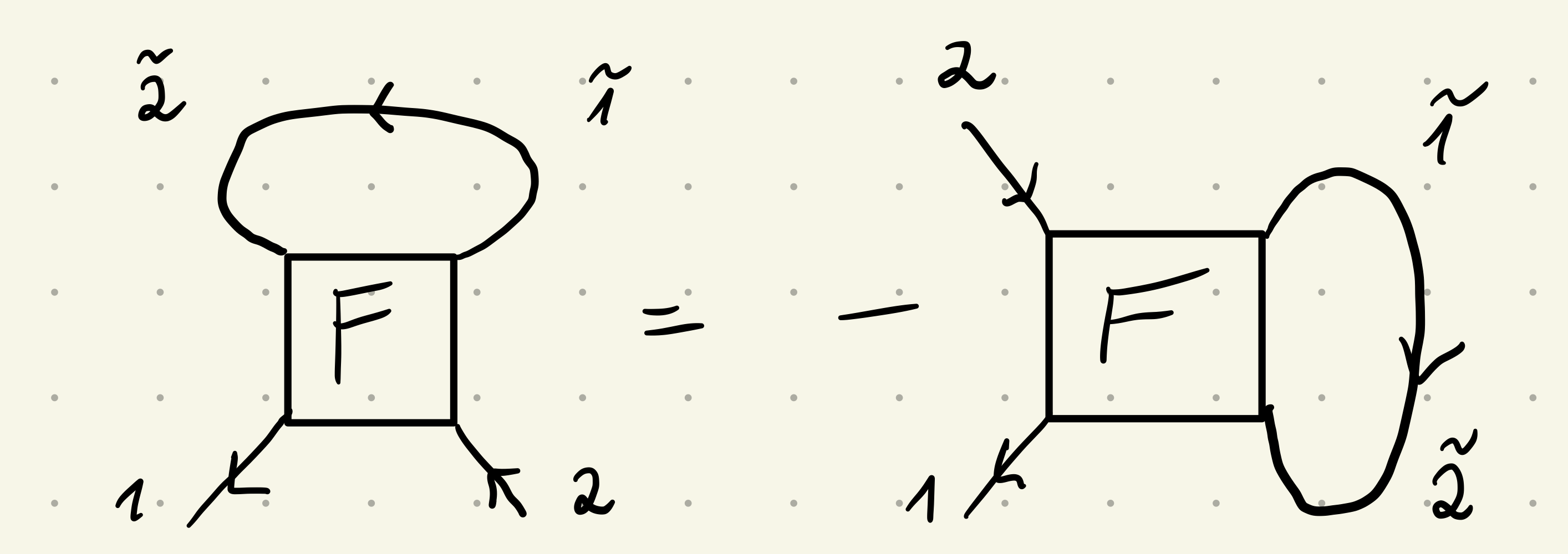
The decomposition of the full vertex into irreducible and reducible parts is powerful, because there exists a set of self-consistent equations for the reducible parts known as the Bethe-Salpeter equations (BSEs). In channel $r$ , the Bethe-Salpeter equation reads

\begin{align} \Phi^r = \Gamma^r \circ \chi^r_0 \circ F \, , \end{align}

(3)

where $\chi^r_0$ is the dressed bubble in channel $r$ (see here) and the symbol ∘ denotes the appropriate contraction of internal variables (momenta, frequencies, spins) depending on the channel $r$ .

An explicit solution of the Bethe-Salpeter equations for $\Phi^r$ can be obtained by iterating them starting from an initial guess (e.g., second order perturbation theory). However, this procedure also requires knowledge of the fully irreducible vertex $\Lambda$ , which is generally unknown. In practice, one therefore often resorts to approximations for $\Lambda$ , such as the parquet approximation, discussed below.

Schwinger-Dyson equation¶

Additionally to the Bethe-Salpeter equations, there exists another exact relation connecting the full vertex $F$ to the self-energy $\Sigma$ , known as the Schwinger-Dyson equation (SDE). Such a relation is required to close the set of equations, since the self-energy is needed to compute the dressed propagators appearing in the bubbles $\chi^r_0$ of the Bethe-Salpeter equations.

The SDE reads

\begin{align} \Sigma_{12} = \zeta F_{0, 1 \tilde{2} \tilde{1} 2} G_{\tilde{2} \tilde{1}} + \frac{1}{2} \zeta F_{0, 1 \tilde{2} \tilde{5} \tilde{4}} G_{\tilde{2} \tilde{1}} G_{\tilde{4} \tilde{3}} G_{\tilde{6} \tilde{5}} F_{\tilde{3} \tilde{6} \tilde{1} 2}\, , \end{align}

(6)

and is represented diagrammatically as

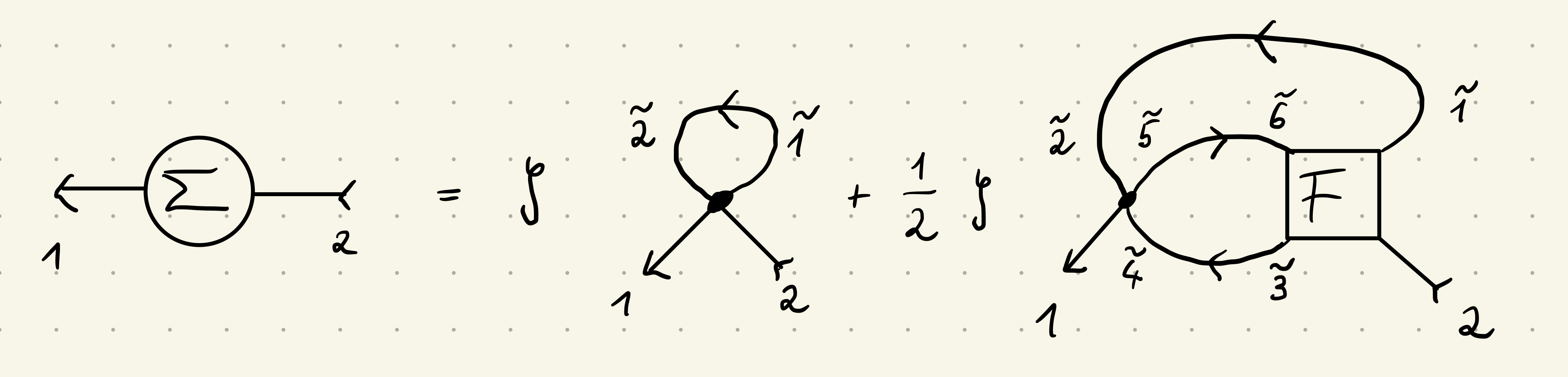
The first term is the Hartree term $\Sigma_\mathrm{H}$ , which yields a static shift of the self-energy. The second, dynamic term, can be written using more compact notation by introducing the loop product $\cdot$ as

\begin{align} [F \cdot G]_{12} = F_{1 \tilde{2} \tilde{1} 2} G_{\tilde{2} \tilde{1}} = \zeta F_{1 2 \tilde{1} \tilde{2}} G_{\tilde{2} \tilde{1}} = \zeta [G \cdot F]_{12} \, . \end{align}

(7)

Employing this notation, the Schwinger-Dyson equation can be written as

\begin{align} \Sigma &= \zeta F_0 \cdot G + \frac{1}{2} \zeta (F_0 \circ \chi^{\overline{ph}}_0 \circ F) \cdot G \\ &= \zeta F_0 \cdot G + \zeta (F_0 \circ \chi^{pp}_0 \circ F) \cdot G \\ &= G \cdot F_0 + \frac{1}{2} G \cdot (F \circ \chi^{ph}_0 \circ F_0) \, , \end{align}

(8)

where we used $\zeta^2 = 1$ in the last line.

Parquet approximation¶

The BSEs and the SDE together form a closed set of equations for the two-particle reducible parts $\Phi^r$ of the vertex $F$ and the self-energy $\Sigma$ , provided that the fully irreducible vertex $\Lambda$ is known. However, $\Lambda$ is generally unknown, so that one has to resort to approximations in practice. One such approximation is the parquet approximation, which consists of approximating the fully irreducible vertex by the bare interaction:

\begin{align} \Lambda = F_0 + \mathcal{O}(F_0^4) \approx F_0 \, . \end{align}

(9)

The parquet approximation has several convenient properties. It

yields the simplest possible solution of the parquet equations
sums up all leading logarithmic divergent terms (in the presence of infrared divergences in loops)
fully includes inter-channel feedback, so there is no ladder bias (unlike in simpler approximations such as RPA)
preserves crossing symmetries
fulfills sum rules for the self-energy and susceptibilities
satisfies the Mermin-Wagner theorem (which states that there can be no long-range order in 2D systems at finite temperature)

However, the parquet approximation also has some drawbacks. In particular, it is a perturbative approximation that fails to hold beyond weak to intermediate coupling strengths. Furthermore, it is not a conserving approximation in the sense of Baym and Kadanoff, which leads to violations of conservation laws and Ward identities.