Starting point: Many-body Hamiltonian and action

We begin with a general many-body Hamiltonian for interacting particles in second quantization, $H[c^\dagger, c]$ , for which the partition function is given by the path integral in imaginary time,

\begin{align} Z &= \int \mathcal{D}[\bar{c}, c] \, e^{-S[\bar{c}, c]} \\ S[\bar{c}, c] &= \int_0^\beta d\tau \left\{ \sum_1 \bar{c}_1(\tau) \partial_\tau c_1(\tau) + H[c_1^\dagger(\tau), c_1(\tau+0^-)] \right\} = S_0 + S_I\, . \end{align}

(1)

The multi-index 1 denotes all quantum numbers of the fields, e.g. momentum, spin, and orbital.

In generic notation, we can write for an arbitrary quartic interaction:

\begin{align} S = S_0 + S_I &= -\sum_{1,2} \bar{c}_1 (G_0)^{-1}_{12} c_2 - \frac{1}{4} \sum_{1,2,3,4} \bar{c}_1 \bar{c}_3 F_{0;1234} c_2 c_4 \, . \end{align}

(2)

Note

$(G_0)^{-1}_{12}$ must be negative definite (i.e. all its eigenvalues must be negative) to ensure convergence of the path integral.
The minus sign in front of the interaction term cancels the minus signs in the expansion of $e^{-S_I}$ .
The sums over multi-indices will be omitted in the future; summation over repeated indices is implied.
$F_0$ is (anti-) symmetric in the arguments: $F_{0;1234} = \zeta F_{0;3214} = \zeta F_{0;1432} = \zeta^2 F_{0;3412}$ , where $\zeta = -1$ for fermions and $\zeta = +1$ for bosons. The factor $(1/2)^2=1/4$ above compensates for summing over terms that are identical due to this crossing symmetry.

About conventions

Different communities use different conventions for numbering the multi-indices. Here, we follow the Vienna convention and use the arabic numbers $(1,2)$ for two-point functions and $(1,2,3,4)$ for four-point functions. In the Munich convention, the action is parametrized as

\begin{align} S = - \bar{c}_{1'} (G_0)^{-1}_{1'1} c_{1} - \frac{1}{4} \bar{c}_{1'} \bar{c}_{2'} F_{0;1'2'|12} c_2 c_1 \, . \end{align}

(3)

When converting between the two conventions, we can therefore use the correspondences

\begin{align} (1,2) &\leftrightarrow (1',1) \\ (1,2,3,4) &\leftrightarrow (1', 2, 2', 1) \, . \end{align}

(4)

Diagrammatically, the bare four-point vertex $F_0$ is represented as the Hugenholtz diagram,

where we number the legs clockwise starting from the bottom left.

The Hamiltonian of the Hubbard model reads

\begin{align} H &= -t \sum_{\langle j, j' \rangle} \sum_{\sigma = \uparrow \downarrow} c^\dagger_{j\sigma} c_{j \sigma} + U \sum_j n_{j\uparrow} n_{j\downarrow} \\ &= \sum_{{\bf k},\sigma} \varepsilon_{\bf k} c^\dagger_{{\bf k}\sigma} c_{{\bf k}\sigma} + U \sum_j c^\dagger_{j\uparrow} c_{j\uparrow} c^\dagger_{j\downarrow} c_{j\downarrow} \end{align}

(5)

With the Fourier transform (see also the chapter on frequency parametrizations)

\begin{align} c_{j\sigma}(\tau) = \frac{1}{\beta}\sum_{i\nu_n} \sum_{\bf k} c_{{\bf k}\sigma}(i\nu_n) e^{i\mathbf{k} \cdot \mathbf{r}_j} e^{-i\nu_n \tau}\, , \end{align}

(6)

the non-interacting parts of the action then reads

\begin{align} S_0 &= \frac{1}{\beta}\sum_{i\nu_n, \mathbf{k}, \sigma} \overline{c}_{\mathbf{k}\sigma}(-i\nu_n) (-i\nu_n + \varepsilon_\mathbf{k}) c_{\mathbf{k}\sigma}(i\nu_n)\, . \end{align}

(7)

The interacting part is usually rewritten by using that $\zeta^2=1$ and suppressing the infinesimal shifts of the imaginary times,

\begin{align} S_I &= U \int_0^\beta d\tau \sum_j \overline{c}_{j\uparrow}(\tau) c_{j\uparrow}(\tau) \overline{c}_{j\downarrow}(\tau) c_{j\downarrow}(\tau) = U \int_0^\beta d\tau \sum_j \overline{c}_{j\uparrow}(\tau) \overline{c}_{j\downarrow}(\tau) c_{j\downarrow}(\tau) c_{j\uparrow}(\tau) \\ &= -\frac{1}{4}\ U \int_0^\beta d\tau_1 d\tau_2 d\tau_3 d\tau_4 \sum_{\substack{j_1, j_2 \\ j_3, j_4}} \sum_{\substack{\sigma_1, \sigma_2 \\ \sigma_3, \sigma_4}} \overline{c}_{j_1 \sigma_1}(\tau_1) \overline{c}_{j_3 \sigma_3}(\tau_3) F_{0; \sigma_1\sigma_2\sigma_3\sigma_4}(\tau_1,\tau_2,\tau_3,\tau_4; j_1, j_2, j_3, j_4) c_{j_2 \sigma_2}(\tau_2) c_{j_4 \sigma_4}(\tau_4)\, , \end{align}

(8)

with the antisymmetrized bare interaction term

\begin{align} &F_{0; \sigma_1\sigma_2\sigma_3\sigma_4}(\tau_1,\tau_2,\tau_3,\tau_4; j_1, j_2, j_3, j_4) \\ &= -U \left(\delta_{\sigma_1, \sigma_4} \delta_{\sigma_3, \sigma_2} - \delta_{\sigma_1, \sigma_2}\delta_{\sigma_3, \sigma_4}\right) \delta_{\sigma_2, \overline{\sigma}_4} \delta(\tau_1=\tau_2=\tau_3=\tau_4) \delta(j_1=j_2=j_3=j_4)\, . \end{align}

(9)

We note in passing that this antisymmetrized bare (Hugenholtz) interaction encompasses both direct and exchange scattering processes. This fact is easily seen by looking at the spin structure of the interaction term,

\begin{align} \overline{c}_{\uparrow} \overline{c}_{\downarrow} c_{\downarrow} c_{\uparrow} &= \frac{1}{2} (\overline{c}_{\uparrow} \overline{c}_{\downarrow} - \overline{c}_{\downarrow} \overline{c}_{\uparrow}) \frac{1}{2} (c_{\downarrow} c_{\uparrow} - c_{\uparrow} c_{\downarrow}) \\ &= \frac{1}{4} (\overline{c}_{\uparrow} \overline{c}_{\downarrow} c_{\downarrow} c_{\uparrow} + \overline{c}_{\downarrow} \overline{c}_{\uparrow} c_{\uparrow} c_{\downarrow} - \overline{c}_{\uparrow} \overline{c}_{\downarrow}c_{\uparrow} c_{\downarrow} - \overline{c}_{\downarrow} \overline{c}_{\uparrow} c_{\downarrow} c_{\uparrow}) \\ &= \frac{1}{4} \sum_\sigma (\overline{c}_{\sigma} \overline{c}_{\bar{\sigma}} c_{\bar{\sigma}} c_{\sigma} - \overline{c}_{\sigma} \overline{c}_{\bar{\sigma}} c_{\sigma} c_{\bar{\sigma}}) \\ &= \frac{1}{4} \sum_{\substack{\sigma_1, \sigma_2 \\ \sigma_3, \sigma_4}} \left(\delta_{\sigma_1, \sigma_4} \delta_{\sigma_3, \sigma_2} - \delta_{\sigma_1, \sigma_2}\delta_{\sigma_3, \sigma_4}\right) \delta_{\sigma_2, \overline{\sigma}_4} \overline{c}_{\sigma_1} \overline{c}_{\sigma_3} c_{\sigma_2} c_{\sigma_4}\, , \end{align}

(10)

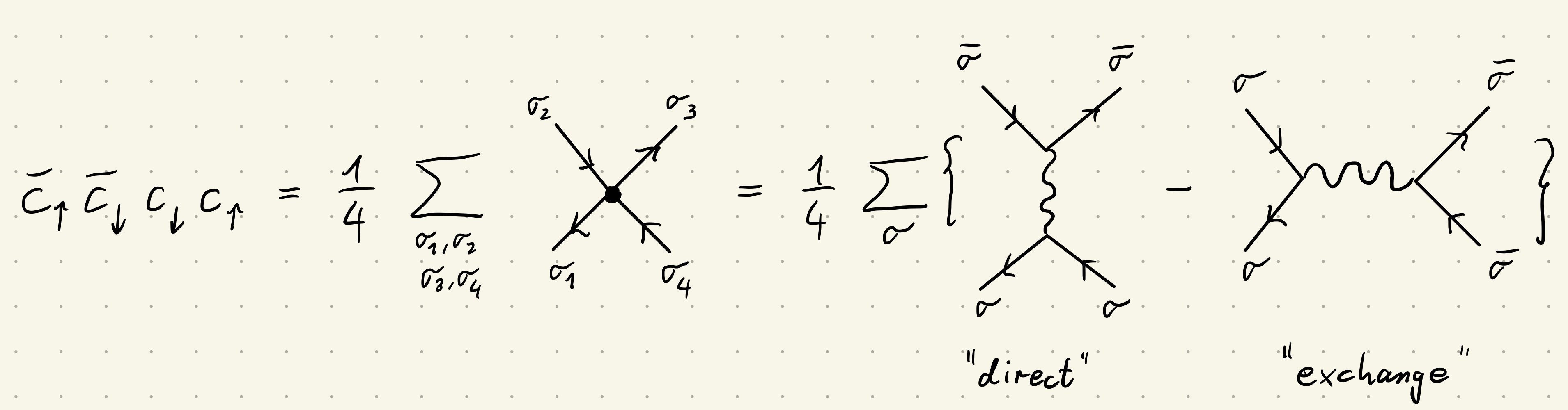
This convenient Hugenholtz notation ultimately leads to a great simplification of all following diagrammatics.

Fourier transforming again with the conventions laid out in the chapter on frequency parametrizations leads to

\begin{align} &F_{0; \sigma_1\sigma_2\sigma_3\sigma_4}(\nu_1,\nu_2,\nu_3,\nu_4; k_1, k_2, k_3, k_4) \\ &= \int_0^\beta d\tau_1 d\tau_2 d\tau_3 d\tau_4 e^{-i\nu_1 \tau_1} e^{-i\nu_2 \tau_2} e^{-i\nu_3 \tau_3} e^{-i\nu_4 \tau_4} \sum_{\substack{j_1, j_2 \\ j_3, j_4}} e^{i k_1 j_1} e^{i k_2 j_2} e^{i k_3 j_3} e^{i k_4 j_4} \\ &\phantom{=} \times F_{0; \sigma_1\sigma_2\sigma_3\sigma_4}(\tau_1,\tau_2,\tau_3,\tau_4; j_1, j_2, j_3, j_4) \\ &= -U \left(\delta_{\sigma_1, \sigma_4} \delta_{\sigma_3, \sigma_2} - \delta_{\sigma_1, \sigma_2}\delta_{\sigma_3, \sigma_4}\right) \delta_{\sigma_2, \overline{\sigma}_4} \int_0^\beta d\tau_1 e^{-i (\nu_1 + \nu_2 + \nu_3 + \nu_4) \tau_1} \sum_{j_1} e^{i (k_1 + k_2 + k_3 + k_4) j_1} \\ &= -U \left(\delta_{\sigma_1, \sigma_4} \delta_{\sigma_3, \sigma_2} - \delta_{\sigma_1, \sigma_2}\delta_{\sigma_3, \sigma_4}\right) \delta_{\sigma_2, \overline{\sigma}_4} \delta(\nu_1 + \nu_2 + \nu_3 + \nu_4) \delta(k_1 + k_2 + k_3 + k_4)\, , \end{align}

(11)

with the proper normalization factors implied.